
European
Commission
European
Commission
Guide to Cost-Benefit Analysis of Investment Projects
Economic appraisal tool for Cohesion Policy 2014-2020
December 2014
Regional and Urban Policy
^ -”jr
Europe Direct is a service to help you find answers to your questions about the European Union.
Freephone number (*):
(*) The information given is free, as are most calls (though some operators, phone boxes or hotels may charge you).
EUROPEAN COMMISSION
Directorate-General for Regional and Urban policy
REGIO DG 02 - Communication
Mrs Ana-Paula Laissy
Avenue de Beaulieu 1
1160 Brussels
BELGIUM
E-mail: regio-publication@ec.europa.eu
Internet: http://ec.europa.eu/regional_policy/index_en.cfm
More information on the European Union is available on the Internet (http://europa.eu). Luxembourg: Publications Office of the European Union, 2015
ISBN 978-92-79-34796-2 doi:10.2776/97516
© European Union, 2015
Reproduction is authorised provided the source is acknowledged.
Printed in Italy
PRiNTED on ELEMENTAL CHLORiNE-FREE BLEACHED paper (ECF)
Economic appraisal tool for Cohesion Policy 2014-2020
European Commission
Directorate-General for Regional and Urban policy
Authors: Davide Sartori (Centre for Industrial Studies [CSIL]), Lead author; Gelsomina Catalano, Mario Genco, Chiara Pancotti, Emanuela Sirtori, Silvia Vignetti (CSIL); Chiara Del Bo (Universita degli Studi di Milano).
Academic Panel Review: Massimo Florio (Universita degli Studi di Milano), Panel Coordinator; Per-Olov Johansson (Stockholm School of Economics), Susana Mourato (London School of Economics & Political Science), Arnold Picot (Ludwig-Maximilians-Universitat, Munich), Mateu Turró (Universitat Politecnica de Catalunya).
Technical advisory: JASPERS acted as technical advisor to DG REGIO for the preparation of this Guide, with a focus on the practical issues related to the CBA of major infrastructure projects. In particular, besides peer reviewing the early drafts of the Guide, JASPERS contributed by highlighting best practice and common mistakes in carrying out CBA as well as with the design and development of the seven case studies included in the Guide. The JASPERS team was composed of experts in all sectors covered by the Guide. It was led by Christian Schempp and Francesco Angelini and included Patrizia Fagiani, Joanna Knast-Braczkowska, Marko Kristl, Massimo Marra, Tudor Radu, Paul Riley, Robert Swerdlow, Dorothee Teichmann, Ken Valentine and Elisabet Vila Jorda.
The authors gratefully acknowledges very helpful comments by Witold Willak, Head of Sector, G.1 Major Project Team, the European Commission Directorate-General for Regional and Urban Policy, who has been in charge of the management of the service, by Mateusz Kujawa, European Commission Directorate-General for Regional and Urban Policy, by the members of the Academic Panel Review, by experts from JASPERS and the European Investment Bank (EIB), as well as participants in the Steering Committee meetings including desk officers from the European Commission Directorates-General for Communications Networks, Content and Technology, for Climate Action, for the Environment, for Energy, for Mobility and Transport, for Regional and Urban Policy and for Research and Innovation.
In some cases, constraints of space, of time, or scope of the Guide have limited the possibility by the authors to fully include all the suggested changes to earlier drafts. The usual disclaimer applies and the authors are responsible for any remaining omissions or errors.
The European Commission and the authors accept no responsibility or liability whatsoever with regard to this text. This material is:
• information of general nature which is not intended to address the specific circumstances of any particular individual or entity;
• not necessarily comprehensive, accurate or up to date. It is not meant to offer professional or legal advice.
Reproduction or translation is permitted, provided that the source is duly acknowledged and no modifications to the text are made.
Quotation is authorised as long as the source is acknowledged along with the fact that the results are provisional.
BAU Business As Usual
CBA Cost-Benefit Analysis
CF Conversion Factor
DCF Discounted Cash Flow
EC European Commission
EIA Environmental Impact Assessment
EIB European Investment Bank
ENPV Economic Net Present Value
ERDF European Regional Development Fund
ERR Economic Rate of Return
ESI European and Structural Investment
EU European Union
FDR Financial Discount Rate
FNPV Financial Net Present Value
FRR(C) Financial Rate of Return of the Investment
FRR(K) Financial Rate of Return on National Capital
GDP Gross Domestic Product
GHG Green House Gas
IWS Integrated Water Supply
LRMC Long Run Marginal Cost
MCA Multi-Criteria Analysis
NACE Statistical classification of economic activities
MS Member State
OP Operational Programme
O&M Operation & Maintenance
PPP Public-Private Partnership
QALY Quality-Adjusted Life Year
SCF Standard Conversion Factor
SDR Social Discount Rate
STPR Social Time Preference Rate
VAT Value Added Tax
VOSL Value of Statistical Life
VOT Value of Time
WTP Willingness-to-pay
WTA Willingness-to-accept
WWTP Waste Water Treatment Plant
349
Evidence-based and successful policy requires making investment decisions based on objective and verifiable methods. This is why the Commission has been continuously promoting the use of Cost-Benefit Analyses (CBA) for major infrastructure projects above €50 million. For the first time, in the 2014-2020 period, the basic rules of conducting CBAs are included in the secondary legislation and are binding for all beneficiaries. In general, the Member States plan to implement over five hundred major projects in the 2014-2020 period.
CBA - that is about measuring in “money terms” all the benefits and costs of the project to society - should become a real management tool for national and regional authorities and therefore we have focused on practical elements in the Guide while keeping abreast of recent developments in the scientific world of welfare economics.

In addition, DG Regional and Urban Policy - together with JASPERS - will establish regular CBA forums for exchanging best practices and experience in carrying out CBAs so that we can continue to improve stakeholders' knowledge and its effective application to specific investment projects. For the sake of creating growth and jobs, Member States' projects financed by the European Structural and Investment Funds need to be completed on time and have to provide expected results to our citizens and enterprises.
I am looking forward to the successful use of EU funding in the coming years to show its added value and role in delivering the Europe 2020 strategy.
Corina Cretu,
European Commissioner for Regional Policy
The present guide to Cost-Benefit Analysis (CBA) of investment projects updates and expands the previous edition of 2008. The guide has been revised with consideration for the recent developments in EU polices and methodology for cost benefit analysis and international best practice, and builds on the considerable experience gained in project preparation and appraisal during the previous programming periods of the cohesion policy.
The objective of the guide reflects a specific requirement for the European Commission to offer practical guidance on major project appraisals, as embodied in the cohesion policy legislation for 2014-2020. As with previous versions, however, the guide should be seen primarily as a contribution to a shared European-wide evaluation culture in the field of project appraisal. Its main objective is to illustrate common principles and rules for application of the CBA approach into the practice of different sectors.
The guide targets a wide range of users, including desk officers in the European Commission, civil servants in the Member States (MS) and in candidate countries, staff of financial institutions and consultants involved in the preparation or evaluation of investment projects. The text is relatively self-contained and does not require a specific background in financial and economic analysis of capital investments. The main change with respect to the previous edition concerns a reinforced operational approach and a stronger focus on the investment priorities of the cohesion policy.
The structure of the guide is as follows.
Chapter one presents the regulatory requirements for the project appraisal process and the related decision on a major project. The project appraisal activity is discussed within the more comprehensive framework of the multi-level governance planning exercise of the cohesion policy and its recent policy developments.
Chapter two discusses the CBA guiding principles, working rules and analytical steps that shall be considered for investment appraisal under EU funds. The proposed methodological framework is structured as a suggested agenda and check-list, both from the standpoint of the investment proposer, who is involved in assessing or preparing a project dossier, and the project examiner involved in project appraisals.
Chapters three to seven include outlines of project analysis by sector, focusing on transport, environment, energy, broadband and research & innovation sectors. The aim is to make explicit those aspects of the CBA that are sector-specific, such as typical economic costs and benefits, evaluation methods, reference periods, etc.
To facilitate the understanding and practical application of CBA in the different sectors covered by the Guide, a number of cases studies are provided. The case studies are solely intended as worked examples of the general methodology described in Chapter 2 and the sector specific methodologies. Although the project examples used in the case studies may be partially based on real projects, these have been simplified and modified in many ways to fit the intended purpose, which is why they are not necessarily representative of the complexity of any real project. Also, the projects selected are only illustrative examples of a vast variety of possible project types within each infrastructure sector and should not be seen as a standard project for the given sector. Similarly, none of the specific assumptions featured in any of the case studies are meant to be seen as representative or standard for any other project, in any sector or country, but rather as illustrative examples. Finally, it should also be noted that for reasons of space limitations in this Guide, the case studies have been generally kept as short as possible and thus many details had to be left out in many ways.
A set of annexes cover the following topics: financial discount rate; social discount rate; approaches for empirical estimation of conversion factors; shadow wage; tariff setting, polluter pays principle and affordability; willingness to pay approach; project performance indicators; probabilistic risk analysis; other appraisal tools. The text is completed by a bibliography.
The EU cohesion policy aims to deliver growth and jobs together with the targets and objectives contained within the Europe 2020 strategy. Choosing the best quality projects which offer best value for money and which impact significantly on jobs and growth is a key ingredient of the overall strategy. In this framework, Cost Benefit Analysis (CBA) is explicitly required, among other elements, as a basis for decision making on the co-financing of major projects included in operational programmes (OPs) of the European Regional Development Fund (ERDF) and the Cohesion Fund.
CBA is an analytical tool to be used to appraise an investment decision in order to assess the welfare change attributable to it and, in so doing, the contribution to EU cohesion policy objectives. The purpose of CBA is to facilitate a more efficient allocation of resources, demonstrating the convenience for society of a particular intervention rather than possible alternatives.
This chapter describes the legal requirements and scope of the CBA in the appraisal of investment projects within the EU cohesion policy, according to the EU regulations and other European Commission documents (see box below). In addition, the role of CBA in the broader framework of EU policy is discussed in light of the EU 2020 Strategy, the targets and objectives of the flagship initiatives and the main sectorial policies and cross cutting issues, including climate change and resource efficiency, in addition to synergies with other EU funding instruments such as the Connecting Europe Facility. The key contents of the chapter are:
• definition and scope of ‘major projects';
• information required, roles and responsibility for the appraisal; and
• consistency with recent policy development and cross cutting issues.
According to Article 100 (Major projects) of Regulation (EU) No 1303/2013, a major project is an investment operation comprising ‘a series of works, activities or services intended to accomplish an indivisible task of a precise economic and technical nature which has clearly identified goals and for which the total eligible cost exceeds EUR 50 million.' The total eligible cost is the part of the investment cost that is eligible for EU co-financing.1 In the case of operations falling under Article 9(7) (Thematic objectives) of Regulation (EU) No 1303/2013, the financial threshold for the identification of major project is set at EUR 75 million.
• Regulation (EU) No 1303/2013 of the European Parliament and of the Council of 17 December 2013 laying down common provisions on the European Regional Development Fund, the European Social Fund, the Cohesion Fund, the European Agricultural Fund for Rural Development and the European Maritime and Fisheries Fund and laying down general provisions on the European Regional Development Fund, the European Social Fund, the Cohesion Fund and the European Maritime and Fisheries Fund and repealing Council Regulation (EC) No 1083/2006.
• Commission Delegated Regulation (EU) No 480/2014 of 3 March 2014 supplementing Regulation (EU) No 1303/2013.
• Commission Implementing Regulation (EU) No 1011/2014 of 22 September 2014 laying down detailed rules for implementing Regulation (EU) No 1303/2013 of the European Parliament and of the Council as regards the models for submission of certain information to the Commission and the detailed rules concerning the exchanges of information between beneficiaries and managing authorities, certifying authorities, audit authorities and intermediate bodies (hereinafter called IR on notification procedure and IQR)
• Commission Implementing Regulation (EU) laying down detailed rules implementing Regulation (EU) No 1303/2013 of the European Parliament and of the Council as regards the models for the progress report, submission of the information on a major project, the joint action plan, the implementation reports for the Investment for growth and jobs goal, the management declaration, the audit strategy, the audit opinion and the annual control report and the methodology for carrying out the cost-benefit analysis and pursuant to Regulation (EU) No 1299/2013 of the European Parliament and of the Council as regards the model for the implementation reports for the European territorial cooperation goal (hereinafter called IR on application form and CBA methodology)
The definition of a major project does not apply to the operation of setting up a financial instrument, as defined by Article 37 (Financial instrument) of Regulation (EU) No 1303/20 1 32, which should undergo a specific procedure3. In the same vein, a Joint Action Plan, as defined by Article 104 (Joint action plan) of Regulation (EU) No 1303/20134 is not a major project. Major projects may be financially supported by the ERDF and Cohesion Fund (hereafter the Funds) as part of an OP or more than one OP (see box below). While the ERDF focuses on investments linked to the context in which firms operate (infrastructure, business services, support for business, innovation, information and communication technologies [ICT] and research applications) and the provision of services to citizens (energy, online services, education, health, social and research infrastructures, accessibility, quality of the environment)5, the Cohesion Fund supports interventions within the area of transport and environment. In the environment field, the Cohesion Fund specifically supports investment in climate change adaptation and risk prevention, investment in the water and waste sectors and the urban environment. Investments in energy efficiency and renewable energy are also eligible for support, provided it has positive environmental benefits. In the field of transport the Cohesion Fund contributes to investments in the Trans-European Transport Network, as well as low-carbon transport systems and sustainable urban transport6.
According to Article 96 (Content, adoption and amendment of operational programmes under the Investment for growth and jobs goal) of Regulation (EU) No 1303/2013, an operational programme shall set out (...) ‘a description of the type and examples of actions to be supported under each investment priority and their expected contribution to the specific objectives referred to in point (i), including the guiding principles for the selection of operations and, where appropriate, the identification of main target groups, specific territories targeted, types of beneficiaries, the planned use of financial instruments and major projects.’
As part of the operational programme(s), the implementation of major projects should be examined by the Monitoring Committee appointed for the specific programme(s) (Article 110). Progress on their preparation and implementation shall be reported in the Annual Implementation Report (Article 111), which Member States are asked to submit annually, from 2016 to 2023.
Financial instruments can be set up to finance major projects, even in combination with ERDF or Cohesion Fund grants. In the latter case separate records must be maintained for each form of financing. In addition, the applicant is asked to specify the type of financial instruments used for financing the project.
In order to get the approval for the co-financing of the major project, the managing authority (MA) of the programme(s) which submits the project is asked to make available the information referred to in Article 101 (Information necessary for the approval of a major project) of Regulation (EU) No 1303/2013 (see box).
(a) Details concerning the body responsible for implementation of the major project, and its capacity.
(b) A description of the investment and its location.
(c) The total cost and total eligible cost, taking account of the requirements set out in Article 61.
(d) Feasibility studies carried out, including options analysis, and the results.
(e) A CBA, including an economic and a financial analysis, and a risk assessment.
(f) An analysis of the environmental impact, taking into account climate change mitigation and adaptation needs, and disaster resilience.
(g) An explanation as to how the major project is consistent with the relevant priority axes of the OP or OPs concerned, and its expected contribution to achieving the specific objectives of those priority axes and the expected contribution to socio-economic development.
(h) The financing plan showing the total planned financial resources and the planned support from the Funds, the EIB, and all other sources of financing, together with physical and financial indicators for monitoring progress, taking account of the identified risks.
(i) The timetable for implementing the major project and, where the implementation period is expected to be longer than the programming period, the phases for which support from the Funds is requested during the programming period.
The information in Article 101(a to i) represents the basis for appraising the major project and determining whether
support from the Funds is justified.
According to Article 102 (Decision on a major project) of Regulation (EU) No 1303/2013, the appraisal procedure can take two different forms. It is up to the Member State to decide which of the two forms to apply for specific major projects under its OPs:
• the first option is an assessment of the major project by independent experts followed by a notification to the Commission by the MA of the major project selected. According to this procedure, the independent experts will assess the information provided on the major project according to Article 101;
• the second option is to send the major project documentation directly to the Commission, in line with the procedure of the 2007-2013 programming period. In this case, the MS shall submit to the Commission the information set out in Article 101, which will be assessed by the Commission.
Regardless of the procedure adopted, the aim is to check that:
• the project dossier is complete, i.e. all the necessary information required by Article 101 is made available and is of sufficient quality;
• the CBA analysis is of good quality, i.e. it is coherent with the Commission methodology; and
• the results of the CBA analysis justify the contribution of the Funds.
The results of the analysis should, in particular, demonstrate that the project is the following:
• consistent with the OP. This is demonstrated by checking that the result(s) produced by the project (e.g. in terms of employment generation, carbon dioxide reduction, etc.) contribute to the specific objective(s) of the priority axis of the programme and policy goals;
• in need of co-financing. This is assessed by the financial analysis and, particularly, with the calculation of the Financial Net Present Value and the Financial Rate of Return of the Investment (FNPV(C) and FRR(C) respectively). To gain a contribution from the Funds, the FNPV(C) should be negative and the FRR(C) should be lower than the discount rate used for the analysis (except for some projects falling under State Aid rules for which this may not be relevant7);
• desirable from a socio-economic perspective. This is demonstrated by the economic analysis result and particularly by a positive Economic Net Present Value (ENPV)8.
In order to assess if the results of the CBA actually support a case for the major project approval, the CBA dossier should demonstrate that the methodology is sound and consistent. To this end, it is of paramount importance that all the information related to the CBA is made easily available and is discussed convincingly by the project beneficiary in the form of a quality CBA report, that refers to methods and tools used (including the model(s) used for calculations) as well as all the working hypotheses underpinning the analysis and especially the forecasts of future values, in addition to their sources. A quality CBA report should therefore be: self-contained (results of previous studies should be briefly recalled and illustrated); transparent (a complete set of data and sources of evidence should be made easily available); verifiable (assumptions and methods used to calculate forecast values should be made available so that the analysis can be replicated by the reviewer); and credible (based on well-documented and internationally accepted theoretical approaches and practices).
Figure 1.1 Role and responsibilities in the Major Project’s appraisal

|
Selection of the appraisal procedure |
1 l 1 | |||
|
/ N X N | ||||
|
S |
s | |||
|
s |
N | |||
|
Li' | ||||
|
\ Art. 102 (1) |
Art. 102 (2) | |||
|
procedure i |
procedure | |||
|
i y |
I y | |||


|
Makes available information referred to in Art.101 to the independent experts |
1 1 Makes available information referred to in Art. 101 and submits an Application Form to the Commission services |
|
1 ] |
1 1 |
|
y |
1 |
|
Assess the project on the basis of the information referred to in Art. 101 and produce an Independent Quality Review report |
| | | | | | | 1 | |
|
i ] y |
] ] ] |
|
r Submits a notification of the selected project to the Commission services |
| |
|
T y |
1 ] V |
|
Assesses the project on the basis of the Independent Quality Review report |
Assesses the project on the basis of the information referred to in Art. 101 with the support of the EIB (if necessary) |
|
] ] V |
] V |
The project is approved/rejected
Source: Authors
Figure 1.2 The role of CBA in the appraisal of the major project
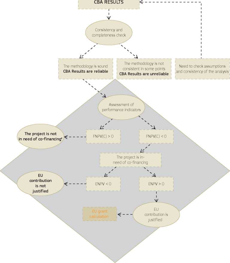
* With exceptions, as set out in Annex III to the Implementing Regulation on application form and CBA methodology. Source: Authors
Where the major project has received a positive appraisal in a quality review by independent experts, according to Article 102(1) (Decision on a major project) of Regulation (EU) No 1303/2013, the Member State may proceed with the selection of the major project and shall notify the Commission. The Commission has 3 months to agree with the independent experts, or adopt the Commission decision refusing the financial contribution to the major project.
If the Commission appraises the major project in accordance with Article 102(2), the Commission shall adopt its decision on the approval (or rejection) of the financial contribution to the selected major project, by means of an implementing act, no later than three months from the date of submission of the information referred to in Article 101.
The co-financing rate for the priority axis, under which the major project is included, shall be fixed by the Commission when adopting the OP [Article 120 (Determination of co-financing rates) of Regulation (EU) No 1303/2013]. For each priority axis, the Commission shall set out whether the co-financing rate for the priority axis is to be applied to the total eligible expenditure (including public and private expenditure) or to the public eligible expenditure. As stated in Article 65 (Eligibility) of Regulation (EU) No 1303/2013, the eligible expenditure of an operation, including major projects, is determined on the basis of national rules ‘except where specific rules are laid down in, or on the basis of, this Regulation or the Fund-specific rules'. Also, specific provisions apply in the case of revenue-generating projects (see box).
The financing method and appraisal procedure of major projects has therefore changed with respect to the 2007-2013 programming period. Table 1.3, displayed at the end of the chapter, highlights the main differences introduced by the new regulations as compared to the Council Regulation 1083/2006.
Revenue-generating projects are investment operations in which discounted revenues are higher than discounted operating costs. According to Article 61 (Operations generating net revenue after completion) of Regulation (EU)
No 1303/2013, the eligible expenditure to be co-financed from the Funds shall be reduced, taking into account the potential of the operation to generate net revenue over a specific reference period that covers both implementation of the operation and the period after completion. The potential net revenue of the operation shall be determined in advance by one of the following methods:
1) Application of a flat rate for the net revenue percentage. It is a simplified approach as compared to the previous programming period.
2) Calculation of discounted net revenue of the operation. This is the method used in the 2007-2013 programming period, in accordance with Article 55 of the Council Regulation 1083/2006.
3) Application of reduced co-financing rates for particular priority axes.
Where it is not objectively possible to determine the revenue in advance according to these methods, Article 61 states that ‘the net revenue generated within three years of the completion of an operation [...] shall be deducted from the expenditure declared to the Commission.’
It should be noted that Article 61 does not apply to operations for which support under the programme constitutes:
(a) de minimis aid; (b) compatible State aid to small and medium-sized businesses (SMEs), where an aid intensity or an aid amount limit is applied in relation to State aid; or (c) compatible State aid, where an individual verification of financing needs in accordance with the applicable State aid rules has been carried out.
For the 2014-2020 programming period, cohesion policy and its Funds are deemed to be a key delivery mechanism to achieve the objectives of Europe 2020 strategy9' As stated in Article 18 (Thematic concentration) of Regulation (EU) No 1303/2013, Member States shall concentrate the EU support (in accordance with the Fund's-specific rules) on actions that bring the greatest added value in relation to the Europe 2020 priorities of smart growth, sustainable growth and inclusive growth.
The EU has set five ambitious targets - in the fields of employment, innovation, education, social inclusion and climate/ energy - which are to be achieved at EU level by 2020. To meet these targets, the Commission proposed a Europe 2020 agenda consisting of seven flagship initiatives representing the investment areas supporting the Europe 2020 priorities. These include: innovation; digital economy; employment; youth; industrial policy; and poverty and resource efficiency.
Actions under the smart growth priority will require investments aimed at strengthening research performance, promoting innovation and knowledge transfer throughout the Union, making full use of ICTs, ensuring that innovative ideas can be turned into products and services that create growth, improving education quality. Investments in specific sectors, such as R&D, ICT and education are considered to be of major strategic importance in the promotion of this objective;
To achieve sustainable growth, it is necessary to invest in operations aimed at limiting emissions and improving resource efficiency. All sectors of the economy, not just emission-intensive ones, are concerned. Environmental measures in water and waste management, investments related to transport and energy infrastructures, as well as instruments based on the use of ICT, are expected to contribute to the shift towards a resource efficient and low-carbon economy. A further step towards sustainable growth will be achieved by supporting manufacturing and service industries (such as tourism) in seizing the opportunities presented by globalisation and the green economy;
Inclusive growth priority requires actions aimed at modernising and strengthening the employment and social protection systems. In particular, this priority specifically addresses the challenge of demographic change by increasing labour participation and reducing structural unemployment (especially for women, young people and older workers). In addition, it will address the challenges of a low skilled workforce and marginalisation (e.g. children and elderly who are particularly exposed to the risk of poverty). In this regard, investments in social infrastructure, including childcare, healthcare, culture and education facilities, will help improve skills. This will enable citizens to balance work with their private lives, and will reduce social exclusion and health inequalities, thus ensuring that the benefits gained from growth can be enjoyed by everyone;
Table 1.1. shows how specific investment sectors are related to the Europe 2020 priorities, flagship initiatives and targets. Within this context, major projects play a key role and their appraisal should be seen as part of a larger planning exercise aimed at identifying the contribution of the project to the achievement of the Europe 2020 strategy. In addition, the projects must comply with EU legislation (e.g. public procurement, competition and State-aid) and sectorial policies.
Finally, all sectors and investments are required to comply with EU climate policy. Climate change issues, both mitigation and adaptation aspects, must be taken into account during the preparation, design and implementation of major projects. That is, major projects shall contribute to the progressive achievement of emissions reduction targets by 2050. Accordingly, in the context of the co-financing request, MAs are required to explain how mitigation and adaptation needs have been taken into account when preparing and designing the project. Second, major projects should be climate-resilient: the possible impacts of the changing climate have to be assessed and addressed at all stages of their development. In the context of the co-funding request, MAs are required to explain which measures have been adopted in order to ensure resilience to current climate variability and future climate change.
Overall, the CBA provides key support in assessing the contribution of the projects to the achievement of Europe 2020 targets. Table 1.2 below shows how certain effects may be identified and quantified through the CBA.
Table 1.1 Matching Investment sectors and Europe 2020 priorities/flagships/targets
|
Europe 2020 priorities |
Europe 2020 flagship initiatives |
Sector/investments |
Europe 2020 targets | ||||
|
Employment |
Innovation |
Climate change |
Education |
Poverty | |||
|
Smart Growth |
Innovation Union |
- Research, Technological Development and Innovation |
V |
V |
V | ||
|
Youth on the move |
- Education |
V |
V | ||||
|
Digital Agenda for Europe |
- ICT |
V |
V | ||||
|
Sustainable Growth |
Resource efficient Europe |
- Environment - Energy - Transport |
V |
V |
V | ||
|
An industrial policy for the globalisation era |
- Entrepreneurship - Industry |
V |
V |
V | |||
|
Inclusive Growth |
An agenda for new skills and jobs |
- Culture - Childcare |
V |
V | |||
|
European Platform against poverty |
- Health - Housi ng |
V | |||||
Source: Authors
Table 1.2 The role of the CBA in contributing towards the achievement of the EU objectives
|
Europe 2020 Targets |
Effects quantifiable through the CBA |
Guide Section |
|
Employment |
The effect, in terms of employment used by the project, is captured by applying the Shadow Wage Conversion Factor to labour cost. The effect, in terms of employment spilling over from the project, is captured by the additional profit created, e.g. by new spin-off companies. |
Par. 2.8.5 Annex IV Par. 7.8.3 |
|
Innovation |
The contribution to the innovation objective is assessed by: - the economic returns generated by license deals; and - the technological progress generated by the project. |
Par. 7.8.3 |
|
Climate change |
The responses to climate change are assessed by estimating costs and benefits of integrating: - climate change mitigation measures, by measuring the economic value of greenhouse gas (GHG) emissions emitted in the atmosphere and the opportunity cost of the energy supply savings; - climate change adaptation measures, resulting from the assessment of the project’s risk-exposure and vulnerability to climate change impacts. |
Par. 2.6.3 Par. 2.8.8 |
|
Education |
The contribution to a higher level of education is assessed by estimating the expected increased income of students and researchers due to better positioning on the job market, as well as the economic value of knowledge outputs (e.g. scientific articles). |
Par. 7.8.4 |
|
Poverty |
Effects on poverty reduction may be assessed by evaluating the equity dimension of the project through the consideration of the households affordability (ability-to-pay), in particular the less wealthy, to access a given public service and the computation of a set of welfare weights. |
Annex V |
Source: Authors
Table 1.3 Main changes compared to the 2007-2013 programming period
|
2007 - 2013 (Regulation 1083/2006) |
2014 - 2020 (Regulation 1303/2013) | |
|
Major project threshold |
Operations where the total cost exceeds EUR 50 million (Art. 39). |
Operations where the eligible cost exceeds EUR 50 million and, in the case of operations contributing to the thematic objective under Article 9(7), EUR 75 million (Art. 100). |
|
Inclusion of major projects in the OP |
The major project is financed as part of an OP or OPs (Art. 39). The list of major projects contained in the OP is indicative. |
The major project is financed as part of an OP or OPs. In addition it can be supported by more than 1 priority axis within the OP. Major projects notified to the Commission under paragraph 1, or submitted for approval under paragraph 2, shall be contained in the list of major projects in an OP (Art. 102). |
|
Project appraisal and decision process |
- Submission: MS submits a major project application to the EC. The COM appraises the major project application on the basis of the information referred in Art. 40 and, if necessary, consulting outside experts including the EIB. - Decision: The Commission adopts a decision within three months. If the Commission appraises the major project and it does not comply with the Regulations, the MS is requested to withdraw the application. Alternatively, the Commission may adopt a negative decision. (Art. 41) |
- Article 102 (1) procedure: at the level of the MS, if the MS decides, the major project is assessed by independent experts supported by technical assistance or, in agreement with the Commission, by other independent experts. The MS notifies the Commission about the results by presenting the information required in Article 101. The Commission approves or refuses the MS’s selection of the major project within three months. In the absence of a decision, the project is deemed approved after three months from its notification (Art. 101). - Article 102 (2) procedure: o The MS sends major project application to the Commission. The Commission appraises and adopts a decision approving or refusing the MS selection of the major project within three months (Art.102). o For an operation which consists of the second or subsequent phase of a major project for which the preceding phase was approved by the Commission and there are no substantial changes compared to the information provided for the major project application submitted in the previous period, in particular as regards the total eligible cost, the MS may proceed with the selection of the major project in accordance with Art. 125(3) and submit the notification containing all the elements, together with confirmation that there are no substantial changes in the major project. No assessment of the information by independent experts is required (Art. 103) |
|
Payment applications |
Expenditure relating to major projects can be included in payment applications before the project has been approved by a Commission decision. |
Expenditure relating to major projects may be included in payment applications only after the MA notifies to the Commission of the major project decision or following the submission for major project application approval. |
|
Validity of Commission approval |
A Commission decision on a major project is valid for the entire programming period. |
Approval by the Commission shall be conditional on the first works/PPP contract being concluded within three years of the date of the approval of the project by the Commission. The deadline could be extended in duly motivated cases by not more than two years. |
|
Calculation of net revenue |
One possibility: - Calculation of discounted net revenues (Art. 55). |
Three possibilities: - Calculation of discounted net revenues - Flat rate net revenue percentage - Decreasing co-financing rate for a chosen priority axis (Art. 61). |
Source: Authors
KJ
4^
GUIDE TO COST-BENEFIT ANALYSIS OF INVESTMENT PROJECTS
Cost-Benefit Analysis (CBA) is an analytical tool for judging the economic advantages or disadvantages of an investment decision by assessing its costs and benefits in order to assess the welfare change attributable to it.
The analytical framework of CBA refers to a list of underlying concepts which is as follows:
• Opportunity cost. The opportunity cost of a good or service is defined as the potential gain from the best alternative forgone, when a choice needs to be made between several mutually exclusive alternatives. The rationale of CBA lies in the observation that investment decisions taken on the basis of profit motivations and price mechanisms lead, in some circumstances (e.g. market failures such as asymmetry of information, externalities, public goods, etc.), to socially undesirable outcomes. On the contrary, if input, output (including intangible ones) and external effects of an investment project are valued at their social opportunity costs, the return calculated is a proper measure of the project's contribution to social welfare.
• Long-term perspective. A long-term outlook is adopted, ranging from a minimum of 10 to a maximum of 30 years or more, depending on the sector of intervention. Hence the need to:
- set a proper time horizon;
- forecast future costs and benefits (looking forward);
- adopt appropriate discount rates to calculate the present value of future costs and benefits;
- take into account uncertainty by assessing the project's risks.
Although, traditionally, the main application is for project appraisal in the ex-ante phase, CBA can also be used for in medias res and ex post evaluation10.
• Calculation of economic performance indicators expressed in monetary terms. CBA is based on a set of
predetermined project objectives, giving a monetary value to all the positive (benefits) and negative (costs) welfare effects of the intervention. These values are discounted and then totalled in order to calculate a net total benefit. The project overall performance is measured by indicators, namely the Economic Net Present Value (ENPV), expressed in monetary values, and the Economic Rate of Return (ERR), allowing comparability and ranking for competing projects or alternatives.
• Microeconomic approach. CBA is typically a microeconomic approach enabling the assessment of the project's impact on society as a whole via the calculation of economic performance indicators, thereby providing an assessment of expected welfare changes. While direct employment or external environmental effects realised by the project are reflected in the ENPV, indirect (i.e. on secondary markets) and wider effects (i.e. on public funds, employment, regional growth, etc.) should be excluded. This is for two main reasons:
- most indirect and/or wider effects are usually transformed, redistributed and capitalised forms of direct effects; thus, the need to limit the potential for benefits double-counting;
- there remains little practice on how to translate them into robust techniques for project appraisal, thus the need to avoid the analysis relies on assumptions whose reliability is difficult to check.
It is recommended, however, to provide a qualitative description of these impacts to better explain the contribution of the project to the EU regional policy goals.11
• Incremental approach. CBA compares a scenario with-the-project with a counterfactual baseline scenario
without-the-project. The incremental approach requires that:
- a counterfactual scenario is defined as what would happen in the absence of the project. For this scenario, projections are made of all cash flows related to the operations in the project area for each year during the project lifetime. In cases where a project consists of a completely new asset, e.g. there is no pre-existing service or infrastructure, the without-the-project scenario is one with no operations. In cases of investments aimed at improving an already existing facility, it should include the costs and the revenues/benefits to operate and maintain the service at a level that it is still operable (Business As Usual12 (BAU)) or even small adaptation investments that were programmed to take place anyway (do-minimum13). In particular, it is recommended to carry out an analysis of the promoter's historical cash-flows (at least previous three years) as a basis for projections, where relevant. The choice between BAU or do-minimum as counterfactual should be made case by case, on the basis of the evidence about the most feasible, and likely, situation. If uncertainty exists, the BAU scenario shall be adopted as a rule of thumb. If do-minimum is used as counterfactual, this scenario should be both feasible and credible, and not cause undue and unrealistic additional benefits or costs. As illustrated in the box below the choice made may have important implications on the results of the analysis;
- secondly, projections of cash-flows are made for the situation with the proposed project. This takes into account all the investment, financial and economic costs and benefits resulting from the project. In cases of pre-existing infrastructure, it is recommended to carry out an analysis of historical costs and revenues of the beneficiary (at least three previous years) as a basis for the financial projections of the with-project scenario and as a reference for the without-project scenario, otherwise the incremental analysis is very vulnerable to manipulation;
- finally, the CBA only considers the difference between the cash flows in the with-the-project and the counterfactual scenarios. The financial and economic performance indicators are calculated on the incremental cash flows only14.
The rest of the chapter presents the conceptual framework of a standard CBA15, i.e. the ‘steps' for project appraisal, enriched with focuses, didactical examples or shortcuts, presented in boxes, to support the comprehension and practical application of the steps proposed. At the end of each section, a review of good practices and common mistakes drawn from empirical literature, ex post evaluations and experience gained from major projects funded during the 2007-13 programming period, is also illustrated. A checklist that can be used as useful tool for checking the quality of a CBA closes the chapter. 11 12 13 14 15
The following example, adapted from EIB (2013)16, illustrates the issue of the project performance in relation to what scenario is selected as counterfactual.
The proposed project, which consists of rehabilitating and expanding existing infrastructure capacity, involves investing EUR 450 million and will result in benefits growing by 5 % per year. The ‘do-minimum’ scenario, which consists of only rehabilitating existing capacity, involves investing EUR 30 million, followed by constant benefits. The BAU involves no investment at all, which, in turn, will affect the amount of output the facility can produce, causing a fall in net benefits of 5 % per year.
As shown below, the results of the CBA change significantly if different scenarios are adopted as counterfactual. By comparing the proposed project with the ‘do-minimum’ scenario, the ERR equals 3 %. If the BAU is taken as a reference, the ERR increases to 6 %. Thus, any choice should be duly justified by the project promoter on the basis of clear evidence about the most feasible situation that would occur in the absence of the project.
|
Scenarios |
EUR m |
NPV |
1 |
2 |
10 |
21 | |
|
1 |
Proposed project |
Net benefit |
1,058 |
45 |
47 |
70 |
119 |
|
Investment |
435 |
450 | |||||
|
2 |
Do-minimum |
Net benefit |
661 |
45 |
45 |
45 |
45 |
|
Investment |
29 |
30 | |||||
|
3 |
Business As Usual |
Net benefit |
442 |
45 |
43 |
28 |
16 |
|
Investment |
0 | ||||||
|
Results | |||||||
|
1-2 |
Proposed project net of Do-minimum |
Net flows |
-9 |
-420 |
2 |
25 |
74 |
|
ERR |
3% | ||||||
|
1-3 |
Proposed project net of Business As Usual |
Net flows |
182 |
-450 |
4 |
42 |
103 |
|
ERR |
6% |
Source: EIB (2013)
Standard CBA is structured in seven steps:
1. Description of the context
2. Definition of objectives
3. Identification of the project
4. Technical feasibility & Environmental sustainability
5. Financial analysis
6. Economic analysis
7. Risk assessment.
The following sections illustrate, in detail, the scope of each step.
Figure 2.1 The steps of the appraisal
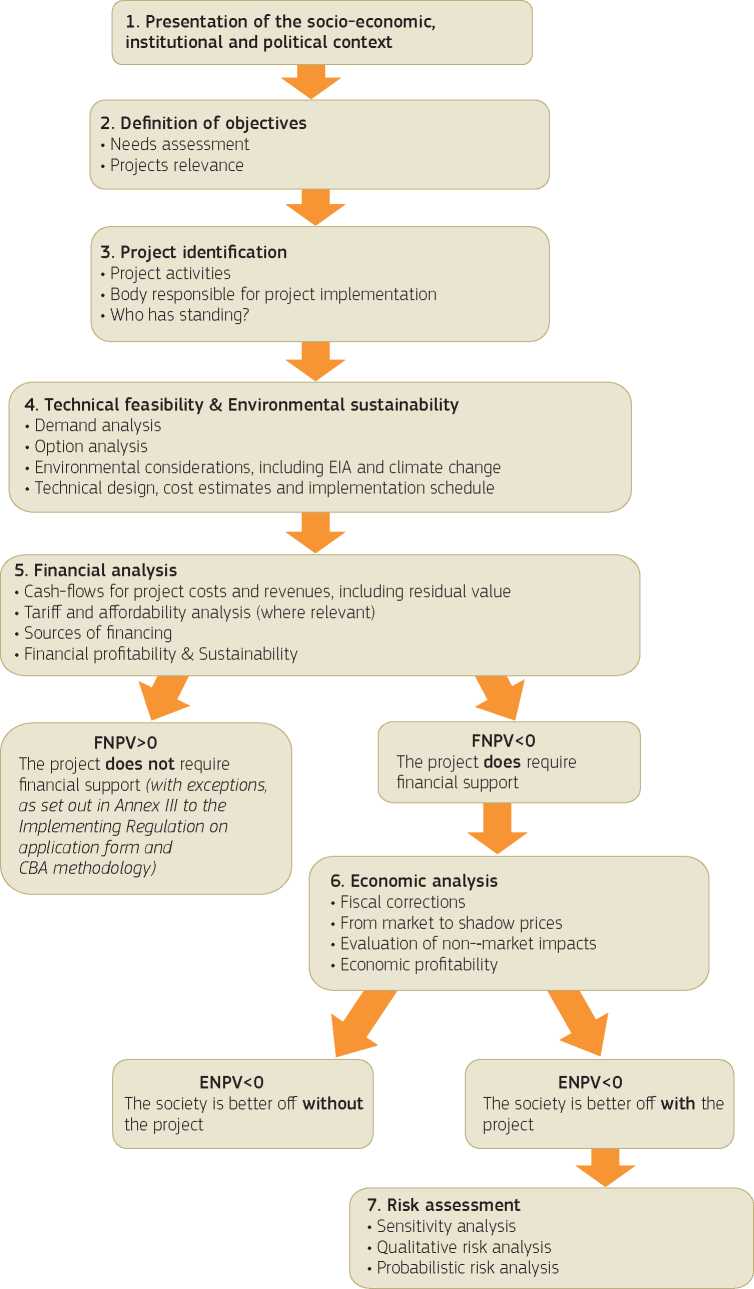
Source: Authors
The first step of the project appraisal aims to describe the social, economic, political and institutional context in which the project will be implemented. The key features to be described relate to:
• the socio-economic conditions of the country/region that are relevant for the project, including e.g. demographic dynamics, expected GDP growth, labour market conditions, unemployment trend, etc.;
• the policy and institutional aspects, including existing economic policies and development plans, organisation and management of services to be provided/developed by the project, as well as capacity and quality of the institutions involved;
• the current infrastructure endowment and service provision, including indicators/data on coverage and quality of services provided, current operating costs and tariffs/fees/charges paid by users, if any17;
• other information and statistics that are relevant to better qualify the context, for instance, existence of environmental issues, environmental authorities likely to be involved, etc.;
• the perception and expectations of the population with relation to the service to be provided, including, when relevant, the positions adopted by civil society organisations.
The presentation of the context is instrumental to forecast future trends, especially for demand analysis. In fact, the possibility of achieving credible forecasts about users, benefits and costs often relies on the assessment's accuracy of the macro-economic and social conditions of the region. In this regard, an obvious recommendation is to check that the assumptions made, for instance on GDP or demographic growth, are consistent with data provided in the corresponding OP or other sectorial and/or regional plans of the Member State.
Also, this exercise aims to verify that the project is appropriate to the context in which it takes place. Any
project is integrated in pre-existing systems with its own rules and features, and this is an imminent complexity that cannot be disregarded. Investments to provide services to citizens can achieve their goals through the integration of either new or renewed facilities into already existing infrastructures. Partnership with the various stakeholders intervening in the system is thus a necessity. Also, sound economic policy, quality institutions and strong political commitment can help the implementation and management of the projects, and the achievement of larger benefits. In short, investments are easier to carry out where the context is more favourable. For this reason, the specific context characteristics need to be taken into due consideration starting from the project design and appraisal phase. In some cases, improvements in the institutional set up might be needed to ensure an adequate project performance.
✓ The context is presented including all sectors that are relevant to the project and avoiding unnecessary discussions on sectors that are unrelated to the project.
✓ The existing infrastructure endowment and service provision is presented with relevant statistics.
✓ The sectorial and regional characteristics of the service to be provided are presented in light of the existing development plans.
X Socio-economic context and statistics are presented without explaining their relevance for the project.
X Socio-economic statistics and forecasts are not based on readily available official data and forecasts.
X The political and institutional aspects are considered irrelevant and not adequately analysed and discussed.
The second step of the project appraisal aims to define the objectives of the project.
From the analysis of all the contextual elements listed in the previous section, the regional and/or sectorial needs that can be addressed by the project must be assessed, in compliance with the sectorial strategy prepared by the MS and accepted by the European Commission. The project objectives should then be defined in explicit relation to needs18. In other words, the needs assessment builds upon the description of the context and provides the basis for the objective's definition.
As far as possible, objectives should be quantified through indicators and targeted19, in line with the result orientation principle of the Cohesion Policy. They may relate, for example, to improvement of the output quality, to better accessibility to the service, to the increase of existing capacity, etc. For a detailed illustration of the typical objectives per sector see chapters three to seven.
A clear definition of the project objectives is necessary to:
• identify the effects of the project to be further evaluated in the CBA. The identification of effects should be linked to the project's objectives in order to measure the impact on welfare. The clearer the definition of the objectives, the easier the identification of the project and its effects. Objectives are highly relevant for the CBA, which should reveal to what extent they are met;
• verify the project’s relevance. Evidence should be provided that the project's rationale responds to a priority for the territory. This is achieved by checking that the project contributes to reaching the EU policy goals and national/regional long-term development plans in the specific sector of assistance. Reference to these strategic plans should demonstrate that the problems are recognised and that there is a plan in place to resolve them.
Whenever possible, the relationship or, better, the relative contribution of the project objectives to achieve the specific targets of the OPs should be clearly quantified. Such identification will also enable the linking of the project objectives with the monitoring and evaluation system. This is particularly important for reporting the progress of major projects in the annual implementation reports, as requested by Article 111 (Implementation reports for the Investment for growth and jobs goal) of Regulation (EU) No 1303/2013. In addition, according to the most recent policy development of the European and Structural
Investment (ESI) Funds, the promoter should also show how and to what extent the project will contribute to achieving the targets of any national or regional sectorial programme.
GOOD PRACTICES
✓ Project effects are identified in clear relation to the project objectives.
✓ The general objectives of the project are quantified with a system of indicators and targets.
✓ Target values are established and compared to the situations with- and without-the-project.
✓ Project indicators are linked to those defined in the respective OP and priority axis. Where the indicators set at the level of the OP are inappropriate to measure the impact of specific projects, additional project-specific indicators, are set up.
✓ If a region or country-wide target exists (e.g. 100 % coverage of water supply in a given service area, diversion of minimum 50 % of biodegradable waste from landfill, etc.), the contribution of the project to achieving this wider target (in % of total target) is explained.
✓ Source and values of indicators are explained.
COMMON MISTAKES
X The economic effects considered in the CBA are not well aligned with the specific objectives of the project.
X Project objectives are confused with its outputs. For instance, if the main objective of the project is to improve the accessibility of a peripheral area, the construction of a new road or the modernisation of the existing network are not objectives, but the means through which the objective of improving the area’s accessibility will be accomplished.
X Where the investment is compliance driven (e.g. UWWTD20), the extent to which the project contributes to achieve such compliance is not shown. If the required standards are not attained by the project, evidence of what other measures are planned and how they will be financed must be provided.
Section 1.2 has presented the legal basis for the definition of a project. Here, some analytical issues involved in project identification are developed. In particular, a project is clearly identified when:
• the physical elements and the activities that will be implemented to provide a given good or service, and to achieve a well-defined set of objectives, consist of a self-sufficient unit of analysis;
• the body responsible for implementation (often referred to as ‘project promoter' or ‘beneficiary') is identified and its technical, financial and institutional capacities analysed; and
• the impact area, the final beneficiaries and all relevant stakeholders are duly identified (‘who has standing?').
A project is defined as ‘as a series of works, activities or services intended in itself to accomplish an indivisible task of a precise economic or technical nature which has clearly identified goals' (Article 100 (Content) of Regulation (EU) No 1303/2013). These works, activities or services should be instrumental in the achievement of the previously defined objectives. A description of the type of infrastructure (railway line, power plant, broadband, waste water treatment plant, etc.), type of intervention (new construction, rehabilitation, upgrade, etc.), service provided (cargo traffic, urban solid waste management, access to broadband for businesses, cultural activities, etc.) and location should be provided in order to define the project activities.
In this regard, the key aspect is that appraisal needs to focus on the whole project as a self-sufficient unit of analysis, which is to say that no essential feature or component is left outside the scope of the appraisal (under-scaling). For example, if there are no connecting roads for waste delivery, a new landfill will not be operational. In that case, both the landfill and the connecting roads are to be considered as a unique project. In general, a project can be defined as technically self-sufficient if it is possible to produce a functionally complete infrastructure and put a service into operation without dependence on other new investments. At the same time, including components in the project that are not essential to provide the service under consideration should be avoided (over-scaling).
The application of this principle requires that:
• partitions of project for financing, administrative or engineering reasons are not appropriate objects of appraisal (‘half a bridge is not a bridge'). A typical case might be that of a request for EU financial support for the first phase of an investment, whose success hinges on the completion of the project as a whole. Or, a request for EU financial support for only a part of a project because the remaining will be financed by other sponsors. In these cases, the whole investment should be considered in CBA. The appraisal should focus on all the parts that are logically connected to the attainment of the objectives, regardless of what the aim of the EU assistance is.
• inter-related but relatively self-standing components, whose costs and benefits are largely independent, should be appraised independently. Sometimes a project consists of several inter-related elements. For example, the construction of a green park area including solid waste management and recreational facilities. Appraising such a project involves, firstly, the consideration of each component independently and, secondly, the assessment of possible combinations of components. The measurement of the economic benefits of individual project components is particularly relevant in the context of large multifaceted projects (see box below). As a whole these projects may present a net positive economic benefit (i.e. a positive ENPV). However, this positive ENPV may include one or more project components that have a negative ENPV. If this component(s) is not integral to the overall project, then excluding it will increase the ENPV for the rest of the project.
• future planned investments should be considered in the CBA if they are critical for ensuring the operations of the original investment. For example, in the case of wastewater treatment, a capacity upgrade of the original plant shall be factored in at a certain point of the project's life cycle, if it is needed to comply with an expected population increase, in order to continue to meet the original project's objectives.
The main driver of the improvement of a railway line is its electrification in order to improve its performance and its integration into the electrified network. Given that the construction works will generate some service disruptions, the project incorporates other actions on the line such as alignment improvements, track reconstruction and the adoption of the ERMTS signalling system. The CBA should consider all these investments and their effects.
EU assistance can be designed to co-finance the reorganisation of some water subnets as part of a broader intervention financed with several sponsors and concerning the entire municipality’s water supply network. The larger intervention should be considered as the unit of the analysis.
A system of integrated environmental regeneration which envisages the construction of several waste water treatment plants and the installation of sewage pipelines and pumping stations in different municipalities can be considered as one integrated project if the single components are integral to the achievement of the environmental regeneration of the impact area.
In the context of urban development, the rehabilitation of city walls and streets in the historical centre of a town should be appraised independently from the rehabilitation and adaptation of buildings for commercial activities in the same area.
The project owner, i.e. the body responsible for project implementation, should be identified and described in terms of its technical, financial and institutional capacity. The technical capacity refers to the relevant staff resources and staff expertise available within the organisation of the project promoter and allocated to the project to manage its implementation and subsequent operation. In the case of the need to recruit additional staff, evidence should be provided that no constraints exist to find the necessary skills on the local labour market. The financial capacity refers to the financial standing of the body, which should demonstrate that it is able to guarantee adequate funding both during implementation and operations. This is particularly important when the project is expected to require substantial cash inflow for working capital or other financial imbalances (e.g. medium-long term loan, clearing cycle of VAT, etc.). The institutional capacity refers to all the institutional arrangements needed to implement and operate the project [e.g. set up of a Project Implementation Unit (PIU)] including the legal and contractual issues for project licensing. Where necessary, special external technical assistance may need to be foreseen and included in the project.
When the infrastructure owner and its operator are different, a description of the operating company or agency who will manage the infrastructure (if already known) and its legal status, the criteria used for its selection, and the contractual arrangements foreseen between the partners, including the funding mechanisms (e.g. collection of tariffs/service fees, presence of government subsides), should be provided.
After having described the project activities and the body responsible for project implementation, the boundaries of the analysis should be defined. The territorial area affected by the project effects is defined as the impact area. This can be of local, regional or national (or even EU) interest, depending on the size and scope of the investment, and the capacity of the effects to unfold. Although generalisations should be avoided, projects typically belonging to some sectors have a common scope of effects. For example, transport investments such as a new motorway (the same does not usually apply to urban transport), even if implemented within a regional framework, should be analysed from a broader perspective since they usually form part of an integrated network that may extend beyond the geographical scope of the analysis. The same can be said for an energy plant serving a delimited territory but belonging to a wider system. In contrast, water supply and waste management projects are more frequently of local interest. However, all projects must incorporate a wider perspective when dealing with environmental issues related to CO2 and other greenhouse gas (GHG) emissions with effects on climate change, which are intrinsically non-local.
A good description of the impact area requires the identification of the project's final beneficiaries, i.e. the population that benefits directly from the project. These may include, for example, motorway users, households exposed to a natural risk, companies using a science park, etc. It is recommended to explain what type of benefits will be enjoyed and to quantify them as much as possible. The identification of the final beneficiaries should be consistent with the assumptions of the demand analysis (see section 2.7.1).
In addition, all bodies, public and private, that are affected by the project need to be described. Large infrastructure investment does not usually only affect the producer and the direct consumers of the service, but can generate larger effects (or ‘reactions') e.g. on partners, suppliers, competitors, public administrations, local communities, etc. For instance, in the case of a high speed train linking two major cities, local communities along the train layout may be affected by negative environmental impacts, while the benefits of the project are accrued by the inhabitants of the larger areas. The identification of ‘who has standing’ should account for all the stakeholders who are significantly affected by the costs and benefits of the project. For a more detailed discussion about how to integrate distributional effects in the CBA see section 2.9.11.
16
✓ Where a project has several stages or phases, these are properly presented together with their respective costs and benefits.
✓ Individual investment measures are bundled into one single project when these are: i) integral to the achievement of the intended objectives and complementary from a functional point of view; ii) implemented in the same impact area; iii) share the same project owner; and iv) have similar implementation periods.
X An artificial splitting of the project is adopted to reduce the project investment cost in order to fit under the major projects threshold.
X Project over-scaling: investments which are functionally independent of each other are packaged together
without a preliminary verification of the economic viability of each investment and of possible combinations and without a clear functional and strategic link among them.
X Project under-scaling: a request for assistance is presented for financing a portion of a project which cannot be justified in isolation from other functional elements.
X Project over-sizing due to over-optimistic assessment of the impact area, e.g. on the basis of unrealistic assumptions of demographic growth.
X The institutional set-up for project operations is presented unclearly.This will make it difficult to verify that financial cash flows are properly accounted for in the financial analysis.
X Benefits of a second phase of a project are included in the economic analysis of the first phase without also including the additional costs, thus making the first phase look economically and/or financially more attractive.
Technical feasibility and environmental sustainability are among the elements of information to be provided in the funding request for major projects (Article 101 (Information necessary for the approval of a major project) of Regulation (EU) No 1303/2013). Although both analyses are not formally part of the CBA, their results must be concisely reported and used as a main data source within the CBA (see box). Detailed information should be provided on:
• demand analysis;
• options analysis;
• environment and climate change considerations;
• technical design, cost estimates and implementation schedule.
In the following, a review of the key information that needs to be summarised in the CBA, in order to understand the overall justification of the project solution sought, is provided. Although they are presented consecutively, they should be viewed as parts of an integrated process of project preparation, where each piece of information and analysis feed each other into a mutual-learning exercise (see box).
The CBA principles should be adopted in the project design process as soon as possible. The CBA should be understood as an ongoing, multi-disciplinary, exercise performed throughout the project preparation in parallel with other technical and environmental considerations. Prerequisites for the CBA of the proposed project solution are, however, the finalisation of a detailed demand analysis and the availability of investment and operational and management (O&M) cost estimates, including costs for environmental mitigation and adaptation measures. These are based on the preliminary project design, which are centrepieces of the ‘technical’ feasibility study and the EIA.
This does not necessarily mean that the analysts responsible for preparing the CBA should start working after the engineers complete the preliminary technical design and deliver the cost estimates, but rather in parallel. In fact, analysts preparing the CBA should adopt an interdisciplinary approach to project preparation from an early stage and are usually involved in preliminary, simplified CBAs for comparisons of different technical and environmental options. Their involvement in the preparation of the demand analysis and options analysis is useful (and often decisive) in achieving the best results for the project.
Once the optimal project solution is identified, a full-scale CBA is usually performed at the end of the preliminary design stage. The aim is to provide confirmation to the project planner(s) of the adequacy and economic convenience of the proposed solution to meet the pre-established project objectives. The results of the full-scale CBA, based on the most recent cost estimates, shall be presented in the EU request for co-financing.
Demand analysis identifies the need for an investment by assessing:
• current demand (based on statistics provided by service suppliers/ regulators/ ministries/ national and regional statistical offices for the various types of users);
• future demand (based on reliable demand forecasting models that take into consideration macro- and socio-economic forecasts, alternative sources of supply, elasticity of demand to relevant prices and income, etc.) in both the scenarios with- and without-the-project.
Both quantifications are essential to formulate demand projections, including generated/induced demand where relevant21, and to design a project with the appropriate productive capacity. For example, it is necessary to investigate which share of the demand for public services, rail transport, or disposal of waste material can be expected to be satisfied by the project. Demand hypotheses should be tested by analysing the conditions of both the present and future supply, which may be affected by actions that are independent from the project.
For a detailed discussion about the main factors affecting demand, methods and outputs of demand analysis in the different fields of intervention see chapters three to seven.
Particular attention should be paid to identifying whether the project under consideration belongs to networks. This is particularly the case for transport and energy infrastructures, which always form part of networks, but also for ICT and telecommunication projects.
When projects belong to networks, their demand (and consequently their financial and economic performance) is highly influenced by issues of mutual dependency (projects might compete with each other or be complementary) and accessibility (ease of reaching the facility).
Several techniques (e.g. multiple regression models, trend extrapolations, interviewing experts, etc.) can be used for demand forecasting, depending on the data available, the resources that can be dedicated to the estimates and the sector involved. The selection of the most appropriate technique will depend, amongst other factors, on the nature of the good or service, the characteristics of the market and the reliability of the available data. In some case, e.g. transport, sophisticated forecast models are required.
Transparency in the main assumptions, as well in the main parameters, values, trends and coefficients used in the forecasting exercise, are matters of considerable importance for assessing the accuracy of the estimates. Assumptions concerning the policy and regulatory framework evolutions, including norms and standards, should also be clearly expressed. Furthermore, any uncertainty in the prediction of future demand must be clearly stated and appropriately treated in risk analysis (see section 2.10). The method used for forecasting, the data source and the working hypotheses must be clearly explained and documented in order to facilitate the understanding of the consistency and realism of the forecasts. Even the information about the mathematical models used, the tools that support them and their qualification, are fundamental elements of transparency.
GOOD PRACTICES
✓ Use is made of appropriate modelling tools to forecast future demand.
✓ Where macro-economic/socio-economic data/forecasts are available from official national sources, consistent use of them is made across all projects/sectors within the country.
✓ Demand is appraised separately for all distinct groups of users/consumers relevant to the project.
✓ Effects of current or planned policy measures and economic instruments that could influence the project are taken into account for demand analysis. Also, all parallel investments potentially affecting the demand for services delivered by the project are identified, described and assessed.
COMMON MISTAKES
X The methodology and parameters used for estimation of current and future demand are not explicitly presented nor justified, or they deviate from national standards and/or official forecasts for the region/country.
X Users’ growth rates ‘automatically’ assumed throughout the entire reference period of the project are
overoptimistic. Where uncertainty exists, it is wise to assume a stabilisation of demand after the first e.g. 3-to-X years of operation.
X Insufficient or incomplete market analysis often leads to an overestimation of revenues. In particular, a full assessment of the competition in the market (projects providing similar products and/or surrogates) and quality requirements for project outputs are often neglected.
X The link between demand analysis and design capacity of the project (supply) is missing or unclear. The design capacity of the project should always refer to the year in which demand is highest.
Undertaking a project entails the simultaneous decision of not undertaking any of the other feasible options. Therefore, in order to assess the technical, economic and environmental convenience of a project, an adequate range of options should be considered for comparison.
Thus, it is recommended to undertake, as a first step, a strategic options analysis, typically carried out at pre-feasibility stage and which may require multiple criteria analysis (see box). The approach for option selection should be as follows:
• establish a list of alternative strategies to achieve the intended objectives;
• screen the identified list against some qualitative criteria, e.g. multi-criteria analysis based on a set of scores22, and identify the most suitable strategy.
- Different routes or construction timing in transport projects (roads/rails).
- Centralised vs. decentralised systems for water supply or wastewater treatment projects.
- A new gravity sewer main and a new wastewater treatment plant vs. a pumping station and pressure pipes that pump the wastewater towards an existing treatment plant, but with a capacity which has to be increased;
- Different locations for a centralised landfill in a regional waste management project.
- Retrofitting an old power plant or building a new one.
- Different peak-load arrangements for energy supply.
- Construction of underground gas storage facilities vs. new LNG terminal.
- Large hospital structures rather than a more widespread offer of health services through local clinics.
- Possible re-use of existing infrastructure (e.g. ducts, poles, sewerage networks) or possible co-deployment with other sectors (energy, transport) to reduce the cost of broadband deployment projects23 24 25 26.
- Different procurement (classic public procurement vs. PPP) and user charging methods for large infrastructures.
Once the strategic option is identified, a comparison of the specific technological solutions is typically carried out at feasibility stage. In some circumstances, it is useful to consider, as a first technological option, a ‘do-minimum' solution. As mentioned, this assumes incurring certain investment outlays, for example for partial modernisation of an existing infrastructure, beyond the current operational and maintenance costs. Hence, this option includes a certain amount of costs for necessary improvements, in order to avoid deterioration of infrastructure or sanctions24. Synergies in infrastructure deployment (e.g. transport/energy and high-speed broadband infrastructure) should also be considered, in view of better use of public funds, higher socio-economic impact, and lower environmental impact.
Once all potential technological solutions are identified, also in the context of the Environmental Impact Assessment (EIA)/ the Strategic Environmental assessment (SEA) procedures and their results (see next paragraph), they need to be assessed and the optimal solution selected as the subject of the financial and economic appraisal. The following criteria shall be applied:
• if different alternatives have the same, unique, objective (e.g. in the case of compliance-driven projects with predetermined policy objectives or targets) and similar externalities, the selection can be based on the least cost solution25 per unit of output produced;
• if outputs and/or externalities, especially environmental impacts, are different in different options (assuming all share the same objective), it is recommended to undertake a simplified CBA for all main options in order to select the best alternative. A simplified CBA usually implies focusing on first qualified estimates of demand and rough estimates of the key financial and economic parameters, including investment and operating costs, the main direct benefit(s) and externalities26. The calculation of the financial and economic performance indicators in the simplified CBA must be made, as usual, with the incremental technique.
The criteria considered in selecting the best solution, with ranking of their importance and the method used in the evaluation, shall always be presented by the project promoter as a justification for the option chosen.
✓ The options analysis is based on a common baseline (i.e. a common counterfactual scenario and consistent demand analysis are adopted across the options).
✓ The options analysis starts from a more strategic point of view (i.e. general type of infrastructure and/or location/alignment for the project) and continues with an assessment of specific technological variants for the type of infrastructure/site selected. New alternative technologies are accompanied by a thorough assessment of their technological, financial, managerial risks, climate risk and environmental impacts.
✓ For comparisons based on costs, all assumptions on unit costs of investment, O&M and replacement should be disclosed and explained separately for each option to facilitate their appraisal. Unit costs of common consumables (e.g. labour, energy, etc.) are the same for all options.
✓ Options are compared using the same reference period.
X The various project options are discussed and analysed in detail, but they are not assessed against a counterfactual scenario which forms the basis of the incremental approach.
X The identification of possible alternatives is done rather ‘artificially’, e.g. alternatives are not genuine solutions but simply constructed to show they are worse than the preferred (pre-decided) alternative.
X There is lack of ‘strategic thinking’: project options are considered only in terms of alternative routes (for
transport projects) or alternative technologies of a pre-selected solution, but not in terms of possible alternative means to achieve the intended objectives.
X Too many or irrelevant criteria, or inappropriate scoring, are used in multi-criteria analysis for shortlisting the project options.
Some requirements on the project's environmental sustainability should be fulfilled in parallel with the technical considerations and contribute to the selection of the best project option.
In particular, the project promoter shall demonstrate to which extent the project: a) contributes to achieve the resource efficiency and climate change targets for 2020; b) complies with the Directive on the prevention and remedying of environmental damage (2004/35/EC); c) respects the ‘polluter pays' principle, the principle of preventive action and the principle that environmental damage should be rectified at source; d) complies with protection of the Natura 2000 sites and protection of species covered by the Habitats Directive (92/43/EEC) and the Birds Directive (2009/147/EC); e) is implemented as a result of a plan or programme falling within the scope of the Strategic Environmental Assessment (SEA) (2001/42/EC); f) is compliant with the Council Directive 2014/52/EU on the Environment Impact Assessment (EIA)27, as well as any other legislation requiring an environmental assessment to be carried out. In addition, environmental investments, e.g. water supply, wastewater and solid waste management, have to comply with other sector-specific Directives, as further illustrated in chapter 4.
When appropriate, an EIA must be carried out to identify, describe and assess the direct and indirect effects of the project on human beings and the environment. While the EIA is a formally distinct and self-standing procedure, its outcomes need to be integrated in the CBA and be in the balance when choosing the final project option. The costs of any environmental integration measures resulting from the EIA procedure (including measures for protection of biodiversity) are treated as input in the assessment of the financial and economic viability of the project. On the other hand, the benefits resulting from such measures are estimated, as far as possible, when valuing the non-market impacts generated by the project (see section 2.9.8).
Impacts of the project on climate, in terms of reduction of GHG emissions, are referred to as climate change mitigation and must be included in the EIA. The following emission sources must be taken into account when assessing the impact of the project on climate:
• direct GHG emissions caused by the construction, operation, and possible decommissioning of the proposed project, including from land use, land-use change and forestry;
• indirect GHG emissions due to increased demand for energy;
• indirect GHG emissions caused by any additional supporting activity or infrastructure which is directly linked to the implementation of the proposed project (e.g. transport, waste management).
On the other hand, the impacts of climate change on the project, referred to as climate change adaptation or resilience to climate change, must also to be addressed during the project design process, when necessary.28 Climate change adaptation is a process aimed to reduce the vulnerability of natural and human systems against actual or expected climate change effects. The main threats to infrastructure assets include damage or destruction caused by extreme weather events, which climate change may exacerbate; coastal flooding and inundation from sea level rise; changes in patterns of water availability; and effects of higher temperature on operating costs, including effects in temperate and/or permafrost29 The following phenomena need to be screened:
• heat waves (including impact on human health, damage to crops, forest fires, etc.);
• droughts (including decreased water availability and quality and increased water demand);
• extreme rainfall, riverine flooding and flash floods;
• storms and high winds (including damage to infrastructure, buildings, crops and forests);
• landslides;
• rising sea levels, storm surges, coastal erosion and saline intrusion;
• cold spells;
• freeze-thaw damage.
To support resilience to climate change in infrastructure investments, the Commission encourages project promoters to assess the project's risk-exposure and vulnerability to climate change impacts. The ‘Guidelines for project managers: Making vulnerable investment climate resilient'30 include a methodology to systematically assess the sustainability and viability of infrastructure projects in changing climate conditions. These guidelines are not intended as a substitute for EIA or CBA, but as a complement to the existing project appraisal tools and development procedures.
Costs and benefits resulting from the integration of both mitigation and adaptation measures in the project design are used in the appraisal of the project's financial and economic performance.
✓ Environment and climate change considerations, including impact assessment on Natura 2000, are incorporated into the project design and preparation at an early stage, i.e. during project screening and scoping. Climate change adaptation and/or mitigation measures are integrated into the EIA procedure together with other environmental impacts.
✓ Cost of measures taken for correcting negative environmental impacts are included in the investment cost considered in the CBA.
✓ Early dialogue between the developer and the authorities/nature experts is carried out to run procedures smoothly and to enable better and faster decisions, which in turn could reduce costs and avoid delays.
X There is no consistency between options analysed in the CBA and options analysed in the EIA. In particular, the option selected in the CBA must have been fully analysed in the EIA.
X Project cost does not incorporate cost of measures related to climate change mitigation, adaptation and other environmental impacts.
X The benefits of mitigation measures are not properly taken into account.
A summary of the proposed project solution shall be presented with the following headings.
• Location: description of the location of the project including a graphical illustration (map). Availability of land is a key aspect: evidence should be provided that the land is owned (or can be accessed) by the beneficiary, who has the full title to use it, or has to be purchased (or rented) through an acquisition process. In the latter case, the conditions of acquisition should be described. The administrative process and the availability of the relevant permits to carry out the works should also be explained.
• Technical design: description of the main works components, technology adopted, design standards and specifications. Key output indicators, defined as the main physical quantities produced (e.g. kilometres of pipeline, number of overpasses, number of trees planted, etc.), should be provided.
• Production plan: description of the infrastructure capacity and the expected utilisation rate. These elements describe the service provision from the supply side. Project scope and size should be justified in the context of the forecasted demand.
• Costs estimates: estimation of the financial needs for project realisation and operations are imported in the CBA as a key input for the financial analysis (see section 2.8). Evidence should be provided as to whether cost estimations are investor estimates, tender prices or out-turn costs.
• Implementation timing: a realistic project timetable together with the implementation schedule should be provided including, for example, a Gantt chart (or equivalent) with the works planned. A reasonable degree of detail is needed in order to enable an assessment of the proposed schedule.
✓ A concise summary of the results of the feasibility study(ies) is included in the CBA report to explain the justification of the selected solution. Input data from the technical studies are duly used in the CBA. Should the FS include a section on CBA, consistency with the main CBA report is ensured or major differences explained.
✓ The technical description of investment and operating cost components provides sufficient detail to allow for cost benchmarking.
As set out in Article 101 (Information necessary for the approval of a major project) of Regulation (EU) No 1303/2013, a financial analysis must be included in the CBA to compute the project's financial performance indicators. Financial analysis is carried out in order to:
• assess the consolidated project profitability;
• assess the project profitability for the project owner and some key stakeholders;
• verify the project financial sustainability, a key feasibility condition for any typology of project;
• outline the cash flows which underpin the calculation of the socio-economic costs and benefits (see section 2.9).
The cash inflows and outflows to be considered are described in detail below. The methods to reduce the eligible expenditure of the operation and calculate the Union assistance (taking into account the potential to generate net revenue) are not discussed in this Guide. Please refer to Art. 61 (operations generating net revenue after completion) of (EU) Regulation 1303/2013 and Article 15 (Method for calculating discounted net revenue) of Commission Delegated Regulation (EU) No 480/2014.
The financial analysis methodology used in this guide is the Discounted Cash Flow (DCF) method, in compliance with section III (Method for calculating the discounted net revenue of operations generating net revenue) of Commission Delegated Regulation (EU) No 480/2014. The following rules should be adopted:
• Only cash inflows and outflows are considered in the analysis, i.e. depreciation, reserves, price and technical contingencies and other accounting items which do not correspond to actual flows are disregarded.
• Financial analysis should, as a general rule, be carried out from the point of view of the infrastructure owner. If, in the provision of a general interest service, owner and operator are not the same entity, a consolidated financial analysis, which excludes the cash flows between the owner and the operator, should be carried out to assess the actual profitability of the investment, independent of the internal payments. This is particularly feasible when there is only one operator, which provides the service on behalf of the owner usually by means of a concession contract.31
• An appropriate Financial Discount Rate (FDR) is adopted in order to calculate the present value of the future cash flows. The financial discount rate reflects the opportunity cost of capital. The practical ways of estimating the reference rate to use for discounting are discussed in Annex I, while the box below reminds the European Commission's reference parameter suggested for the programming period 2014-2020.
• Project cash-flow forecasts should cover a period appropriate to the project's economically useful life and its likely long term impacts. The number of years for which forecasts are provided should correspond to the project's time horizon (or reference period). The choice of time horizon affects the appraisal results. In practice, it is therefore helpful to refer to a standard benchmark, differentiated by sector and based on internationally accepted practice. The Commission-proposed reference periods are shown in table 2.1. These values should be considered as including the implementation period. In the case of unusually long construction periods, longer values can be adopted.
• The financial analysis should usually be carried out in constant (real) prices, i.e. with prices fixed at a base-year. The use of current (nominal) prices [i.e. prices adjusted by the Consumer Price Index (CPI)] would involve a forecast of CPI that does not seem always necessary. When a different rate of change of relative prices is envisaged for specific key items, this differential should be taken into account in the corresponding cash flow forecasts.
On the other hand, when there are many operators, the consolidation of the analysis might not be feasible. In this case, the analysis perspective should be that of the project promoter, either owner or operator, depending on the investment typology (see for example section 3.7.3 in the Transport chapter).
• When the analysis is carried out at constant prices, the FDR will be expressed in real terms. When the analysis is carried out at current prices, a nominal FDR will be used31.
• The analysis should be carried out net of VAT, both on purchase (cost) and sales (revenues), if this is recoverable by the project promoter. On the contrary, when VAT is not recoverable, it must be included.32
• Direct taxes (on capital, income or other) are considered only for the financial sustainability verification and not for the calculation of the financial profitability, which is calculated before such tax deductions. The rationale is to avoid capital income tax rules complexity and variability across time and countries.
According to Article 19 (Discounting of cash flows) of Commission Delegated Regulation (EU) No 480/2014, for the programming period 2014-2020, the European Commission recommends that a 4 % discount rate in real terms is considered as the reference parameter for the real opportunity cost of capital in the long term. Values differing from the 4 % benchmark may, however, be justified on the grounds of international macroeconomic trends and conjunctures, the Member State’s specific macroeconomic conditions and the nature of the investor and/or the sector concerned. To ensure consistency amongst the discount rates used for similar projects in the same country, the Commission encourages the Member States to provide their own benchmark for the financial discount rate in their guidance documents and then to apply it consistently in project appraisal at national level.
Table 2.1 European Commission’s reference periods by sector
|
Sector |
Reference period |
|
(years) | |
|
Railways |
30 |
|
Roads |
25-30 |
|
Ports and airports |
25 |
|
Urban transport |
25-30 |
|
Water supply/sanitation |
30 |
|
Waste management |
25-30 |
|
Energy |
15-25 |
|
Broadband |
15-20 |
|
Research and Innovation |
15-25 |
|
Business infrastructure |
10-15 |
|
Other sectors |
10-15 |
Source: ANNEX I to Commission Delegated Regulation (EU) No 480/2014.
The financial analysis is carried out by a set of accounting tables, as illustrated in Figure 2.2. and in table 2.2, and, in more detail, in the following sections.
Figure 2.2 Structure of financial analysis
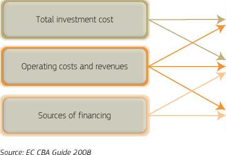
Financial return on investment - FNPV(C)
Financial sustainability
Financial return on capital - FNPV(K)
Table 2.2 Financial analysis at a glance
|
FNPV(C) |
SUSTAINABILITY |
FNPV(K) | |
|
Investment costs | |||
|
Start-up and technical costs |
- |
- | |
|
Land |
- |
- | |
|
Buildings |
- |
- | |
|
Equipment |
- |
- | |
|
Machinery |
- |
- | |
|
Replacement costs |
- |
- |
-* |
|
Residual value |
+ |
+ | |
|
Operating costs | |||
|
Personnel |
- |
- |
- |
|
Energy |
- |
- |
- |
|
General expenditure |
- |
- |
- |
|
Intermediate services |
- |
- |
- |
|
Raw materials |
- |
- |
- |
|
Other outflows | |||
|
Loan repayments |
- |
- | |
|
Interests |
- |
- | |
|
Taxes |
- | ||
|
Inflows | |||
|
Revenues |
+ |
+ |
+ |
|
Operating subsidies |
+ | ||
|
Sources of financing | |||
|
Union assistance |
+ | ||
|
Public contribution |
+ |
_** | |
|
Private equity |
+ |
- | |
|
Private loan |
+ |
* Only if they are self-financed by the project revenues. Otherwise, if new sources of financing (either equity or debt) are needed to sustain them, these sources must be displayed within the outflows at the time they are disbursed.
** Operating subsidies shall not be accounted in order to avoid double counting with the operating costs outflow.
Source: Adapted from EC CBA Guide 2008.
The first step in the financial analysis is the analysis of the amount and breakdown over the years of the total investment costs. Investment costs are classified by:
• Initial investment: it includes the capital costs of all the fixed assets (e.g. land, constructions buildings, plant and machinery, equipment, etc.) and non-fixed assets (e.g. start up and technical costs such as design/planning, project management and technical assistance, construction supervision, publicity, etc.). Where appropriate, changes in net working capital should also be included. Information must be taken from the technical feasibility study(ies)33 and the data to consider are the incremental cash disbursements encountered in the single accounting periods (usually years) to acquire the various types of assets (see box). Cost breakdown over the years should be consistent with the physical realisations envisaged and the time-plan for implementation (see section 2.7.4)34. Where relevant, the initial investment shall also include environmental and/or climate change mitigating costs during the construction, as usually defined in the EIA or in other appraisal procedures.
• Replacement costs: includes costs occurring during the reference period to replace short-life machinery and/or equipment, e.g. engineering plants, filters and instruments, vehicles, furniture, office and IT equipment, etc.35 36 37
It is preferable not to compute cash-flows for large replacements close to the end of the reference period. When a specific project asset needs to be replaced shortly before the end of the reference period, the following alternatives should be considered:
• shorten the reference period to match the end of the design lifetime of the large asset that needs replacing;
• postpone the replacement until after the end of the reference period and assume an increase of the annual maintenance and repair cost for the specific asset until the end of the reference period.
According to the incremental approach, investment costs should be considered net of possible avoided capital costs in the counterfactual scenario. The latter costs are based on the assumption that, without the investment, there is no longer a feasible situation so that it is in any case necessary to implement other interventions, at least in a way to guarantee a minimum level of service provision. This is the assumption of taking the do-minimum as the reference scenario (see section 2.2). For example, in the electrical sector, a new substation could be needed to satisfy the load increase in the absence of a new line. This cost must be included in the counterfactual scenario.
A residual value of the fixed investments must be included within the investment costs account for the end-year. The residual value reflects the capacity of the remaining service potential of fixed assets whose economic life is not yet completely exhausted.37 The latter will be zero or negligible if a time horizon equal to the economic lifetime of the asset has been selected.
According to Article 18 (Residual value of the investment) of Commission Delegated Regulation (EU) No 480/2014, for project assets with economic lifetimes in excess of reference period, their residual value shall be determined by ‘computing the net present value of cash flows in the remaining life years of the operation'38 Other residual value calculation methods may be used in duly justified circumstances. For instance, in the case of non-revenue generating projects38, by computing the value of all assets and liabilities based on a standard accounting depreciation formula39 40 41 or considering the residual market value of the fixed asset as if it were to be sold at the end of the time horizon. Also, the depreciation formula should be used in the special case of projects with very long design lifetimes, (usually in the transport sector), whose residual value will be so large as to distort the analysis if calculated with the net present value method.
The residual value can be singled out either within the project inflows or within the investment costs but with negative sign (see table 2.3 for an example).
Table 2.3 Total investment costs. EUR thousands
|
Years | ||||||||
|
Total |
1 |
2 |
3 |
4-9 |
10 |
11-29 |
30 | |
|
Start-up and technical costs |
6,980 |
1,816 | ||||||
|
Land |
1,485 |
757 | ||||||
|
Buildings |
37,342 |
17,801 | ||||||
|
Equipment |
11,355 |
23,273 | ||||||
|
Machinery |
25,722 | |||||||
|
Initial Investment |
126,531 |
8,465 |
75,176 |
42,890 | ||||
|
Replacement costs |
1 |
11,890 |
9,760 | |||||
|
Residual value |
i |
f |
-4,265 | |||||
|
Total Investment costs |
152,655 |
8,465 |
75,176 |
42,890 |
_L |
11,890 |
9,760 |
-4,265 |
These can include also costs, e.g. for feasibility studies, borne before the start of the evaluation period, although not eligible for EU funding.
In the example, expenditures of EUR 11.9 and 9.8 million are expected in year 10 and 20, respectively, to replace short life equipment and machinery.
The residual value is considered with negative sign because it is an inflow.
The second step in financial analysis is the calculation of the total operating costs and revenues (if any).
Operating costs41 include all the costs to operate and maintain (O&M) the new or upgraded service. Cost forecasts can be based on historic unit costs, when patterns of expenditures on operations and maintenance ensured adequate quality standards.42 Although the actual composition is project-specific, typical O&M costs include: labour costs for the employer; materials needed for maintenance and repair of assets; consumption of raw materials, fuel, energy, and other process consumables; services purchased from third parties, rent of buildings or sheds, rental of machinery; general management and administration; insurance cost; quality control; waste disposal costs; and emission charges (including. environmental taxes, if applicable).
These costs are usually distinguished between fixed (for a given capacity, they do not vary with the volume of good/service provided) and variable (they depend on the volume).
Cost of financing (i.e. interest payments) follow a different course and must not be included within the O&M costs.
The change of relative prices is defined as the total nominal increase (decrease) rate net of the inflation (deflation) factor, as defined by the CPI.
When the prices of some input and output items are expected to change significantly, above or below the average inflation rate, this differential should be taken into account in the corresponding cash flow forecasts.
Since there is high uncertainty over price evolution in the long term, the application of changes of relative prices should, however, be the result of proper analysis and supporting evidence should be provided in the CBA. For example, increase rates applied across all O&M costs and of the same magnitude must be avoided. In particular, high real increases of unit costs of both energy (e.g. fuel and electricity) and labour are not plausible as these together determine an large amount of average inflation. Also, with regards to labour costs, any assumed increase in real salaries and wages can be partially offset by increases in labour productivity throughout the time horizon.
The project revenues are defined as the ‘cash in-flows directly paid by users for the goods or services provided by the operation, such as charges borne directly by users for the use of infrastructure, sale or rent of land or buildings, or payments for services' (Article 61 (Operations generating net revenue after completion) of (EU) Regulation 1303/2013).
These revenues will be determined by the quantities forecasts of goods/services provided and by their prices. Incremental revenues may come from increases in quantities sold, in the level of prices, or both.
Transfers or subsidies (e.g. transfers from state or regional budgets or national health insurance), as well as other financial income (e.g. interests from bank deposits) shall not be included within the operating revenues for the calculations of financial profitability because they are not directly attributable to the project operations42. On the contrary, they shall be computed for the financial sustainability verification.
When the contribution of the state or other public authority (PA) is, however, in exchange for a good or service directly provided to it by the project (i.e. the state is the user), this shall be generally considered a project revenue and included in the financial profitability analysis. In other words, it is not relevant how the state or PA pays for the goods or services (i.e. through tariffs, shadow tolls, availability payments, etc.) because the contribution to the project originates from a direct relation to the use of the project infrastructure.
For compliance with the regulatory requirements, where relevant tariffs shall be fixed in compliance with the polluter-pays and the full-cost recovery principles. In particular, compliance with the polluter-pays principle requires that:
• applied user charges and fees recover the full cost, including capital costs, of environmental services;
• the environmental costs of pollution, costs of resource depletion, and preventive measures are borne by those who cause pollution/ depletion;
• charging systems are proportional to the social marginal production costs which include the full costs, including capital costs, of environmental services, the environmental costs of pollution and the preventive measures implemented and the costs linked to the scarcity of the resources used.
Compliance with the full-cost recovery principle includes that:
• tariffs aim to recover the capital cost, the operating and maintenance cost, including environmental and resource costs;
• the tariff structure maximises the project's revenues before public subsidies, while taking affordability into account.
However, when relevant, e.g. for a project supplying a public service in the environmental sector, affordability considerations should be taken into account in the application of the polluter-pays and the full-cost recovery principles. Key aspects regarding their application and the relative affordability implications are discussed in Annex V.
As shown in table 2.4, the cash outflows of operating costs deducted from the cash flows of revenues determine the net revenues of the project. These are calculated for each year until the time horizon. According to Article 61 Reg. 1303/2013, for the purpose of the EU contribution calculation ‘operating cost-savings generated by the operation shall be treated as net revenue unless they are offset by an equal reduction in operating subsidies'.
Table 2.4 Operating Revenues and Costs. EUR thousands
|
Years | |||||||||||
|
Total |
1-3 |
4 |
5 |
6 |
29 |
30 | |||||
|
Service 1 |
0 |
11,355 |
11,423 |
11,492 |
11,979 |
11,979 | |||||
|
Service 2 |
0 |
243 |
243 |
243 |
243 |
243 | |||||
|
Total revenues |
407,862 |
0 |
11,598 |
11,666 |
11,735 |
12,222 |
12,222 | ||||
|
Personnel |
0 |
1,685 |
1,685 |
1,685 |
1,685 |
1,685 | |||||
|
Energy |
0 |
620 |
623 |
626 |
648 |
648 | |||||
|
General expenditure |
0 |
260 |
260 |
260 |
260 |
260 | |||||
|
Intermediate services |
0 |
299 |
299 |
299 |
299 |
299 | |||||
|
Raw materials |
0 |
2,697 |
2,710 |
2,724 |
2,821 |
2,821 | |||||
|
Total operating costs |
153,487 |
0 |
5,561 |
5,577 |
5,594 |
5,713 |
5,713 | ||||
|
Net revenues |
254,375 |
0 |
6,037 |
6,089 |
6,140 |
6,509 |
6,509 | ||||
|
During the construction phase no operating revenues and costs usually occur. |
ms Personnel costs are assumed to be fixed along the reference period, while energy requirements are variable and follow the expected production growth. | ||||||||||
The next step is the identification of the different sources of financing that cover the investment costs. Within the framework of EU co-financed projects, the main sources can be:
• Union assistance (the EU grant);
• national public contribution (including, always, the counterpart funding from the OP plus additional grants or capital subsidies at central, regional or local government level, if any);
• project promoter's contribution (loans or equity), if any;
• private contribution under a PPP, (equity and loans) if any.
Here, the loan is an inflow and it is treated as a financial resource coming from third parties. Table 2.5 below provides an illustrative example including contributions from private investors.
Table 2.5 Sources of financing. EUR thousands
|
Years | ||||||||
|
Total |
1 |
2 |
3 |
4 |
5 |
6 |
7-30 | |
|
Union assistance |
47,054 |
3,148 |
27,956 |
15,950 |
- |
- |
- |
- |
|
Public contribution |
47,054 |
3,148 |
27,956 |
15,950 |
- |
- |
- |
- |
|
Private equity |
16,212 |
1,085 |
9,632 |
5,495 |
- |
- |
- |
- |
|
Private loan |
16,212 |
1,085 |
9,632 |
5,495 |
- |
- |
- |
- |
|
Total resources |
126,531 |
8,465 |
75,176 |
42,890 |
0 |
0 |
0 |
0 |
|
The Union assistance is calculated in line with the provisions of Art. 61 of Reg. 1303/2012 and by applying a 50 % maximum co-financing rate of the priority axis. |
In the example, the private financing is given by 50 % equity and 50 % loan. |
The total sources of financing should always match the initial investment cost. |
Determination of investment costs, operating costs, revenues and sources of financing enables the assessment of the project profitability, which is measured by the following key indicators:
• financial net present value - FNPV(C) - and financial rate of return - FRR(C) - on investment;
• financial net present value - FNPV (K) - and the financial rate of return - FRR (K) - on national capital.
Return on investment
The financial net present value of investment (FNPV(C)) and the financial rate of return of the investment (FRR(C)) compare investment costs to net revenues and measure the extent to which the project net revenues are able to repay the investment, regardless of the sources or methods of financing.
The Financial net present value on investment is defined as the sum that results when the expected investment and operating costs of the project (discounted) are deducted from the discounted value of the expected revenues:
n
FNPV(C) = =
t=o
Ą |
(1+0° (l+O1
Sn
0+0"
where: St is the balance of cash flow at time t, at is the financial discount factor chosen for discounting at time t and i is the financial discount rate.
The financial rate of return on investment is defined as the discount rate that produces a zero FNPV, i.e. FRR is given by the solution of the following equation43:
o=y—®—
*-i(i+frr)‘
The FNPV(C) is expressed in money terms (EUR), and must be related to the scale of the project. The FRR(C) is a pure number, and is scale-invariant. Mainly, the examiner uses the FRR(C) in order to judge the future performance of the investment in comparison to other projects, or to a benchmark required rate of return. This calculation also contributes to deciding if the project requires EU financial support: when the FRR(C) is lower than the applied discount rate (or the FNPV(C) is negative), then the revenues generated will not cover the costs and the project needs EU assistance. This is often the case for public infrastructures, partly because of the tariff structure of these sectors.
43
The return on investment is calculated considering:
• (incremental) investment costs and operating costs as outflows;
• (incremental) revenues and residual value as inflows.
Thus, cost of financing is not included in the calculation of the performance of the investment FNPV(C) (but is included in the table for the analysis of the return on capital FNPV (K), see below).
Moreover, as mentioned above, capital, income or other direct taxes are included only in the financial sustainability table (see below) and not considered for the calculation of the financial profitability, which is calculated before deductions.
Table 2.6 Calculation of the return on investment. EUR thousands
|
Years | ||||||||
|
1 |
2 |
3 |
4 |
5-9 |
10 |
11-29 |
30 | |
|
Total revenues |
11,598 |
12,011 |
12,222 | |||||
|
Residual value |
4,265 | |||||||
|
Total inflows |
0 |
0 |
0 |
11,598 |
12,011 |
16,487 | ||
|
Total operating costs |
5,561 |
5,662 |
5,713 | |||||
|
Initial Investment |
8,465 |
75,176 |
42,890 | |||||
|
Replacement costs |
11,890 |
9,760 | ||||||
|
Total outflows |
8,465 |
75,176 |
42,890 |
5,561 |
17,552 |
5,713 | ||
|
Net cash flow |
-8,465 |
-75,176 |
-42,890 |
6,037 |
-5,540 |
10,774 | ||
|
FNPV(C) |
- 34.284 | |||||||
|
FRR(C) |
1.4% | |||||||
A financial discount rate of 4 % has been applied to calculate this value.
Return on national capital
The objective of the return on national capital calculation is to examine the project performance from the perspective of the assisted public, and possibly private, entities in the MS (‘after the EU grant').
The return on national capital is calculated considering as outflows: the operating costs; the national (public and private) capital contributions to the project; the financial resources from loans at the time in which they are reimbursed; the related interest on loans. As far as replacement costs are concerned, if they are self-financed with the project revenues, they will be treated as operating costs (as in table 2.7). Otherwise, if new sources of financing (either equity or debt) are needed to sustain them, these sources will be displayed within the outlays at the time they are disbursed. The inflows are the operating revenues only (if any) and the residual value. Subsidies granted to cover operating costs shall be excluded because they are transfers from one to another national source44. Table 2.9 shows this account and readers may see, by comparison with table 2.6 that the former focuses on sources of national funds, while the latter focuses on total investment costs, with the remaining items being identical.
The financial net present value of capital, FNPV(K), in this case, is the sum of the net discounted cash flows that accrue to the national beneficiaries (public and private combined) due to the implementation of the project. The corresponding financial rate of return on capital, FRR(K), of these flows determines the return in percentage points.
When computing FNPV(K) and FRR(K), all sources of financing are taken into account, except for the EU contribution. These sources are taken as outflows (they are inflows in the financial sustainability account), instead of investment costs (as it forms part of the financial return on investment calculation).
While the FRR(C) is expected to be very low, or negative for the public investments to be financed with EU funds, the FRR (K) will be higher and, in some cases, even positive. On the other hand, for public infrastructure, a negative FNPV(K) after EU assistance does not mean that the project is not desirable from the operator's or the public's perspective and should be cancelled. It just means that it does not provide an adequate financial return on national capital employed, based on the benchmark applied (i.e. 4 % in real terms). This is actually a quite common result, even for revenue generating projects receiving EU assistance. In such cases it is particularly important to ensure the financial sustainability of the project.
When relevant, the return on the project promoter's capital (either public or private) can also be calculated45. This compares the net revenues of the investment with the resources provided by the promoter: i.e. the investment cost minus the non-reimbursable grants received from the EU or the national/regional authorities. This exercise can be particularly useful in the context of state aid in order to verify that the intensity of the aid (EU and national assistance) provides the best value for-money with the objective of limiting public financial support to the amount necessary for the project to be financially viable. In fact, when the project expects a substantial positive return (i.e. significantly above the national benchmarks on expected profitability in the given sector) it shows that the grants received would bring supra-normal profits to the beneficiary.
Table 2.7 Calculation of the return on national capital. EUR thousands
|
Years | ||||||||
|
1 |
2 |
3 |
4 |
5-9 |
10 |
11-29 |
30 | |
|
Total revenues |
11,598 |
12,011 |
12,222 | |||||
|
Residual value |
4,265 | |||||||
|
Total inflows |
0 |
0 |
0 |
11,598 |
12,011 |
16,487 | ||
|
Public contribution |
3,148 |
27,956 |
15,950 | |||||
|
Private equity |
1,085 |
9,632 |
5,495 | |||||
|
Loan repayment (including interest) |
1,789 |
1,789 |
1,789 | |||||
|
Total operating & replacement costs |
5,561 |
17,552 |
5,713 | |||||
|
Total outflows |
4,233 |
37,588 |
21,445 |
5561 |
19,341 |
5,713 | ||
|
Net cash flow |
-4,233 |
-37,588 |
-21,445 |
6,037 |
-7,329 |
10,774 | ||
|
FNPV(K) |
11,198 | |||||||
|
FRR(K) |
5.4 % | |||||||
The loan is here an outflow and is only included when reimbursed. In this example, it is assumed to be paid back in ten constant payments starting in year 5.
In this example, replacement costs are self-financed with the project revenues. Accordingly, they are treated as operating costs.
The project is financially sustainable when the risk of running out of cash in the future, both during the investment and the operational stages, is expected to be nil. Project promoters should show how the sources of financing available (both internal and external) will consistently match disbursements year-by-year. In the case of non-revenue generating projects (i.e. not subject to the requirements set out in Article 61 of Regulation (EU) No 1303/2013), or whenever negative-cash-flows are projected in the future (i.e. in years in which large capital investments are required for asset replacements), a clear long-term commitment to cover these negative cash flows must be provided46.
The difference between inflows and outflows will show the deficit or surplus that will be accumulated each year. Sustainability occurs if the cumulated generated cash flow is positive for all the years considered (table 2.8). The inflows include:
• sources of financing;
• operating revenues from the provision of goods and services; and
• transfer, subsidies and other financial gains not stemming from charges paid by users for the use of the infrastructure. The residual value should not be taken into account unless the asset is actually liquidated in the last year of the analysis. The dynamics of the inflows are measured against the outflows. These relate to the following:
• initial investment
• replacement costs
• operating costs
• reimbursement of loans and interest payments
• taxes on capital/income and other direct taxes.
It is important to ensure that the project, even if assisted by EU co-financing, does not risk suffering from a shortage of capital. In particular, in the case of significant reinvestments/upgrades, proof of disposal of sufficient resources to cover these future costs should be provided in the sustainability analysis. In this sense it is recommended to carry out a risk analysis that takes into account the possibility of the key factors in the analysis (usually construction costs and demand) being worse than expected (see Annex VIII).
Table 2.8 Financial sustainability. EUR thousands
|
Years | ||||||||
|
1 |
2 |
3 |
4 |
5-9 |
10 |
11-29 |
30 | |
|
Sources of financing |
8,465 |
75,176 |
42,890 | |||||
|
Total revenues |
11,598 |
12,011 |
12,222 | |||||
|
Total inflows |
8,465 |
75,176 |
42,890 |
11,598 |
12,011 |
12,222 | ||
|
Initial investment |
8,465 |
75,176 |
42,890 | |||||
|
Replacement costs |
11,890 |
9,760 | ||||||
|
Loan repayment (including interest) |
1,789 |
1,789 |
1,789 | |||||
|
Total operating costs |
5,561 |
5,662 |
5,713 | |||||
|
Taxes |
604 |
-733 |
651 | |||||
|
Total outflows |
8,465 |
75,176 |
42,890 |
5,561 |
19,341 |
5,713 | ||
|
Net cash flow |
0 |
0 |
0 |
6,037 |
-7,329 |
6,509 | ||
|
Cumulated net cash flow |
0 |
0 |
0 |
6,037 |
... |
20,726 |
133,835 | |
Financial sustainability is verified if the cumulated net cash flow row is greater than zero for all the years considered.
The cumulated cash flow should be zero (or positive) during the construction phase
If projects fall within an already existing infrastructure, such as capacity extension projects, the overall financial sustainability of the infrastructure operator, including the project (more than that of the single extended segment), should be checked after the project (i.e. in the scenario ‘with the project’), even if the analysis of incremental cash-flows shows that the project will not run out of cash-flow. This is to ensure that not only the project but also the operator will not run out of cash-flow, or possibly experience negative cash flows, after implementation of the project, and is particularly relevant in the case of infrastructure that has previously suffered from severe underfunding.
EU co-financed investment projects may be partly financed by private investors. PPP may be an important tool for financing investment projects when there is appropriate scope to involve the private sector. In order to attract private investors, who generally have different aims, aspirations and a higher aversion to risk than public bodies, proper incentives should be provided, but up to an amount which is not granting an unduly high revenue.
Many types of PPP exist, usually dependent on the specificities and characteristics of each project. The most common PPP models are: Private Operation and Maintenance; Design Build Operate (DBO); Parallel Co-finance of capex; Design, Build, Finance and Operate (DBFO)47. Attention should be paid to the structure of the PPP as it may affect the project's eligible expenditure. In particular, the degree of risk transfer to the private sector changes under each model project type, ranging from models with limited risk transfer (e.g. operation and maintenance risk) through to models with higher risk transfer (e.g. design, construction, financing and operations risk). The following steps shall be considered in the financial analysis of major projects implemented as a PPP:
• Under PPP, the public partner is usually, but not always, the owner of the infrastructure and the private partner is the operator obtaining revenues through tariff payments. A consolidated analysis should first be carried out in order to calculate the overall investment profitability.
• The return on capital shall then be calculated separately for the private partner and public partner:
- in order to check profitability of the private capital to avoid unduly high profit generated by the EU support, the rate of return on private equity - FRR(Kp) - shall be calculated comparing all the revenues accrued by the private partner, net of the operational costs48 borne, including the concession fee (if any), with the financial resources provided during investment (either through equity or loans) (see table 2.9). The results shall be compared with national benchmarks on expected profitability in the given sector. Whenever the private partner is selected on the basis of the most economically advantageous tender criterion, through open public procurement, it is expected that such alignment with national benchmarks is automatically fulfilled;
- a similar exercise can be replicated to calculate the rate of return on public equity - FRR(Kg) - which compares the revenues accrued by the public partner, usually coming from the concession fee, net of the managerial costs of the contract, with the resources provided during investment (either through equity or loans). The result should be compared with the financial discount rate in order to ensure the project is not over-financed.
Table 2.9 Calculation of the return on private equity. EUR thousands
|
Years | ||||||||
|
1 |
2 |
3 |
4 |
5-9 |
10 |
11-29 |
30 | |
|
Total revenues |
11,598 |
12,011 |
12,222 | |||||
|
Total inflows |
0 |
0 |
0 |
11,598 |
12,011 |
12,222 | ||
|
Private equity |
1,085 |
9,632 |
5,495 | |||||
|
Loan repayment (including interest) |
1,789 |
1,789 |
1,789 | |||||
|
Total operating & replacement costs |
5,561 |
17,552 |
5,713 | |||||
|
Concession fee |
1,800 |
1,800 |
1,800 | |||||
|
Total outflows |
1,085 |
9,632 |
5,495 |
7,361 |
21,141 |
7,513 | ||
|
Net cash flow |
-1,085 |
-9,632 |
-5,495 |
4,237 |
-9,129 |
4,709 | ||
|
FNPV(Kp) |
26,806 | |||||||
|
FRR(Kp) |
14.2% | |||||||
A concession fee is usually included within the costs borne by the private operator.
The residual value is excluded because in many PPP contracts the infrastructure is returned to the public sector at the end of the period.
✓ Price and technical contingencies are excluded from the investment cost for the financial profitability calculation, although they are eligible costs (up to 10 % of the initial investment cost).
✓ The inflation rate is based on official national projections of the Consumer Price Index (CPI).
✓ For O&M costs fixed and variable components are calculated separately.
✓ In the counterfactual case, the chosen regime of regular and periodic maintenance and operations does not lead to disproportionate losses of operational performance. Any predicted change of operational performance is shown to realistically correspond to the chosen maintenance and operations regime and to related incremental benefits calculations (such as time savings and modal shift).
✓ Fixed maintenance costs are expressed in % of the net cost of the assets for both civil works and plant components. Variable maintenance costs are expressed in unit cost per output of assets (e.g. EUR/ton, EUR/km, etc.).
✓ When a project adds new assets to complement a pre-existing service or infrastructure, both additional contributions from existing users and contributions from new users of the new service/infrastructure are taken into account to determine the project revenues.
X Replacement costs are not considered in the calculation of residual values.
X The total investment cost in the CBA or its individual elements is inconsistent with the values presented in the feasibility study or in other more advanced engineering design documents, if available.
X Costs for protection of archaeological remains in the project site, as well as environmental and/or climate change integration measures are not included in the project cost.
X VAT is included in the financial analysis even though it is recoverable.
X Asset depreciation, interest and loan repayments, VAT and income tax, and dividends paid to shareholders are included within the O&M costs.
X Subsides received to cover (part of) the operating costs are included in the calculation of the EU contribution as revenues.
X Charges levied by governments in exchange for the goods or services rendered are confused with transfer payments and excluded from the operating revenues. For instance, a charge paid by farmers to the irrigation authority. Although the charge is called ‘tax’, this is not a transfer but a charge directly paid by users in exchange for the use of water. Accordingly, it must be considered as a project’s revenue. Another example is the ‘taxes’ paid by the citizens for waste collection and disposal services.
X In the FRR(K) calculation, cash-flows relative to replacement costs are computed twice: as operating outlays and as equity contribution from the project promoter.
X In the case of loans involved in project financing, loan conditions are not explained.
X Nominal interest rates are used to calculate the interest payments, where the analysis is carried out at constant prices.
As set out in Article 101 (Information necessary for the approval of a major project) of Regulation (EU) No 1303/2013, an economic analysis must be carried out to appraise the project's contribution to welfare49. The key concept is the use of shadow prices to reflect the social opportunity cost of goods and services, instead of prices observed in the market, which may be distorted. Sources of market distortions are manifold (see also Annex III):
• non-efficient markets where the public sector and/or operators exercise their power (e.g. subsidies for energy generation from renewable sources, prices including a mark-up over the marginal cost in the case of monopoly, etc.);
• administered tariffs for utilities may fail to reflect the opportunity cost of inputs due to affordability and equity reasons;
• some prices include fiscal requirements (e.g. duties on import, excises, VAT and other indirect taxes, income taxation on wages, etc.);
• for some effects no market (and prices) are available (e.g. reduction of air pollution, time savings).
The standard approach suggested in this guide, consistent with international practice, is to move from financial to economic analysis. Starting from the account for the return on investment calculation, the following adjustments should be:
• fiscal corrections;
• conversion from market to shadow prices;
• evaluation of non-market impacts and correction for externalities.
After market prices adjustment and non-market impacts estimation, costs and benefits occurring at different times must be discounted. The discount rate in the economic analysis of investment projects, the Social Discount Rate (SDR), reflects the social view on how future benefits and costs should be valued against present ones. Annex II discusses the empirical approaches used for SDR estimation and provides examples of estimates at country level.
According to Annex III to the Implementing Regulation on application form and CBA methodology, for the programming period 2014-2020 the European Commission recommends that for the social discount rate 5 % is used for major projects in Cohesion countries and 3 % for the other Member States. Member States may establish a benchmark for the SDR which is different from 5% or 3 %, on the condition that: i) justification is provided for this reference on the basis of an economic growth forecast and other parameters; ii) their consistent application is ensured across similar projects in the same country, region or sector. The Commission encourages MSs to provide their own benchmarks for the SDR in their guidance documents, possibly at the start of the operational programmes and then to apply it consistently in project appraisal at national level.
Source: EC (2014)
After the use of the appropriate SDR, it is possible to calculate the project economic performance measured by the following indicators: Economic Net Present Value (ENPV), Economic Rate of Return (ERR) and benefit/cost ratio (B/C ratio). In the following sections the steps to move from financial to economic analysis are described.
Taxes and subsidies are transfer payments that do not represent real economic costs or benefits for society as they involve merely a transfer of control over certain resources from one group in society to another. Some general rules can be established to correct such distortions:
• prices for input and output must be considered net of VAT;
• prices for input should be considered net of direct50 and indirect taxes;
• prices (e.g. tariffs) used as a proxy for the value of outputs should be considered net of any subsidy and other transfer granted by a public entity51.
As concerns the methods of eliminating transfer payments, if it is possible to determine their exact value, they should be directly eliminated from the cash flows. For example, VAT payments on construction costs can be simply dropped off in the economic analysis. If it is not possible to determine their exact value, they should be eliminated from the project cash flows using conversion factors (see section 2.8.4).
In some projects the fiscal impact can be significant because, for example, the revenues generated by the project may decrease the need to finance budgetary deficits by public debt or taxation.52
Despite the general rule, in some cases indirect taxes (or subsidies) are intended as a correction for externalities.
For example, taxes on NOx emissions to discourage negative environmental externalities. In this and in similar cases, it is justified to include these taxes (subsidies) in project costs (benefits), provided that they adequately reflect the underlying marginal cost (Willingness-To-Pay (WTP)), but the appraisal should avoid double counting (e.g. including both energy taxes and estimates of full external environmental costs).
When market prices do not reflect the opportunity cost of inputs and outputs, the usual approach is to convert them into shadow prices to be applied to the items of the financial analysis. A simplified operational approach for the estimation of the shadow prices is presented in the Figure below.
Figure 2.3 From market to shadow prices
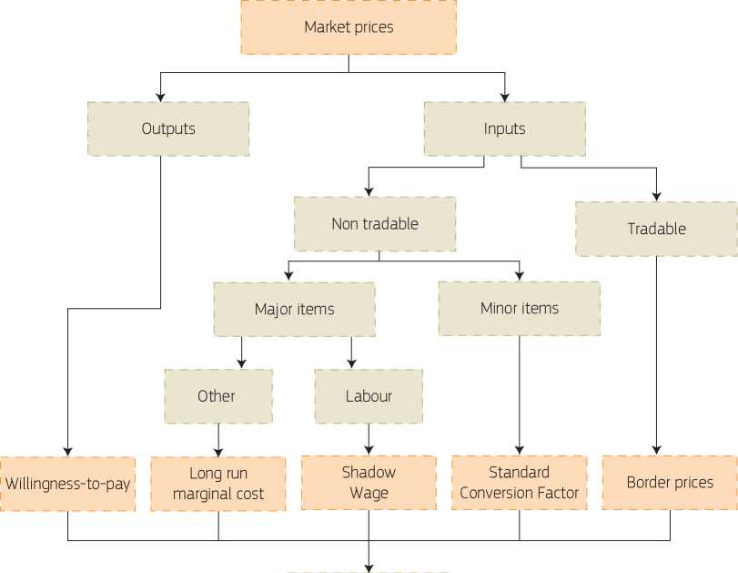
i
Shadow prices
i___________|
Source: Adapted from Saerbeck (1990)
In practice, the following (simplified) operational approach can be applied to convert financial items into shadow prices. Project inputs:
• if they are tradable goods, border prices are used54. If a project uses an imported input, e.g. gas and oil, the shadow price is the import cost plus insurance and freight (CIF) in more liberalised (i.e. competitive and undistorted) markets, thus excluding any custom duties or taxes applied once the good enters the national market. Border prices can be expressed as a percentage of the price of the goods, as a fixed amount per unit or as a minimum price applied as soon as the good passes the border. Where the relevant economic border lies is a matter to be ascertained on a case-by-case basis. In the context of the EU funds, the external border of the EU may be considered relevant for most goods.
• If they are non-tradable goods:
- the Standard Conversion Factor, which measures the average difference between world and domestic prices of a given economy (see box for an example) is applied in the case of ‘minor' items, e.g. administrative costs, intermediate services, etc.; 53
- ad hoc assumptions, depending on the specific hypotheses made on market conditions, should be undertaken in the case of ‘major' items, e.g. land54, civil works, machinery, equipment, etc. to reflect their long run marginal cost55;
- for manpower, the Shadow Wage is calculated.
The method generally used to operationally put into practice the different techniques presented above is to apply a set of conversion factors to the project financial costs. Section 2.9.5 below briefly presents the implications of this practice, while for a more detailed discussion about the existing empirical approaches to convert project inputs into shadow prices see Annex III. The shadow wage is treated separately in section 2.9.6 and in Annex IV.
Project outputs:
• Users' marginal Willingness-To-Pay (WTP), which measures the maximum amount consumers are willing to pay for a unit of a given good, is used to estimate the direct benefit(s) related to the use of the goods or services rendered by the project.
Section 2.9.7 shows the operational approach that should be followed to quantify the project outputs at users' WTP. Annex VI discusses, in detail, the current techniques to estimate WTP and the scope for application.
An illustrative computation of the Standard Conversion Factor (SCF) for a hypothetical country is hereby presented. As shown in Annex III, the simplified formula for the estimation of the SCF is:
SCF = (M+X)/ (M+X+TM)
where: M is the total value of import at shadow prices, i.e. CIF prices; X is the total value of export at shadow prices, i.e. FOB prices; TM is the total value of duties on import.
It is assumed that the total value of export at FOB prices and of import at CIF prices, in a given year, including both intra-EU and extra-EU trade of all products and services, are respectively EUR 25,000 million and EUR 20,000 million.
In the same year, the national general government and the EU collect EUR 500 million as taxes and duties on imports, excluding VAT. Export taxes, duties and other monetary compensatory amounts on exports are nil, as well as import and export subsidies.
International trade detailed data and main national accounts tax aggregates are provided both by Eurostat and national statistics institutes. Hence, in this example:
M= EUR 25,000 million
X= EUR 20,000 million
TM= EUR 500 million.
25,000+20,000
SCF 0.989
The SCF formula leads to the following result: 25,000+20,000+500
The variables in the SCF formula generally do not undergo significant variations on a yearly basis. For this reason the SCF could be either computed for a single year, or as an average of a number of years.
Transforming inputs market prices into shadow prices is completed, in practice, through the application of Conversion Factors. These are defined as the ratio between shadow prices and market prices. They represent the factor at which market prices have to be multiplied to obtain inflows valued at shadow price. Formally:
vi
ki= — ^Vi = Jii-Pi
where: pi are market prices for the good i, v are shadow prices for the same good and k are the conversion factors.
If the conversion factor for one good is higher than one, then the observed price is lower than the shadow price, meaning that the opportunity cost of that good is higher than that captured by the market. Conversely, if the conversion factor is lower than one, then the observed price is higher than the shadow price, due to taxes or other market distortions which add to the marginal social value of a good and determine a higher market price.
In principle, Conversion Factors should be made available by a planning office and not calculated on a project-by-project basis. When national parameters are not available, project-specific calculations can be made but these must then be consistent across projects56. At least, corrections should be applied to depurate market prices from fiscal factors, e.g. an excise tax on import. The following box provides an example.
In the absence of evidence of market failures, the CFs should be set equal to 1.
As an example, let us assume that concrete is an input cost of the investment project. If the unit price of concrete used for the project is EUR 10,000, of which 20 % is VAT57 and import tax rate is 7 % (regardless of the country of origin), a simplified way to estimate the shadow price is to use the conversion factor (CF) computed as follows:
CF = U-/m-VAT)
where / is the import tax rate of the input good entering the CBA. Thus, the shadow price (SP) can be estimated by multiplying the CF by the observed market price (MP) of this good:
SP = (1-/m-VAT)*MP
The CF will amount to CF= (1-0.07)*(1-0.2) =0.93*0.8 =0.744 and the shadow price would be equal to SP=0.744*10,000=7,440.
Since the import tax rate could differ depending on the type of good considered, in order to compute the shadow price of the aggregated item ‘materials’ the project appraiser could use the average tax rate applying to those materials which are more commonly used in investment projects, such as bricks, iron, tubes, concrete, bituminous materials, plastics and other chemical products (e.g. paints), wood, etc. The same approach can also be applied for other cost items. As suggested in Annex III, the Input-Output matrix or the Use Table of a given economy can be used to breakdown aggregated input factors such as civil works, equipment, materials, etc. into their main sub-components, in order to disentangle the traded components to which the border price rule applies, and then compute the conversion factor as a weighted average.
Current wages may be a distorted social indicator of the opportunity cost of labour because labour markets are imperfect, or there are macroeconomic imbalances, as revealed particularly by high and persistent unemployment or by dualism and segmentation of labour conditions (e.g. when there is an extensive informal or illegal economy). The project promoter, in such cases, may resort to a correction of observed wages and to the use of conversion factors for computing shadow wages.
- In the private sector, labour costs for a private company may be lower than the social opportunity cost because the State gives special subsidies to employment in some areas.
- There may be legislation fixing a minimum legal wage, even if due to heavy unemployment there may be people willing to work for less.
- There are informal or illegal sectors with no formal wage or income, but with a positive opportunity cost of labour.
The shadow wage measures the opportunity cost of labour. Typically, in an economy characterised by extensive unemployment or underemployment, this may be less than the actual wage rates paid. In particular:
• for skilled workers previously employed in similar activities, the shadow wage can be assumed equal or close to the market wage;
• for unskilled workers drawn to the project from unemployment, it can be assumed equal to or not less than the value of unemployment benefits or other proxies when unemployment benefits do not exist;
• for unskilled workers drawn to the project from informal activities, it should be equal to the value of the output forgone in these activities.
The methodology to estimate the shadow wage at the national/regional level is illustrated in Annex IV, providing an example of computation which refers to year 2011. Member States are encouraged to develop their own national/regional benchmarks following the approach depicted in the Annex. In the absence of national/regional data, a shortcut formula for determination of the shadow wage is illustrated in the box below.
A practical solution to determine the shadow wage can be the reduction of unit labour costs by a percentage determined by the share of income taxation: SW = W*(l-t)
where: SW is the shadow wage, W is the market wage and t is the income taxation.
If a country is suffering from a high unemployment rate, the shadow wage may be inversely correlated to the level of unemployment. The following formula might be adopted for unskilled manpower used on project construction sites in order to take into account an ‘unemployment effect’, i.e. the excess supply of labour compared to the market clearing level in the case of a persistently high unemployment: SW = W*(1-t)*(1-u)
where: u is the unemployment rate of the region.
For more detailed SW formulas at regional level see Del Bo et al. (2011).
The concept of marginal WTP is commonly used to estimate the shadow price of the project output. In other words, to evaluate the project direct benefits, related to the use of the goods or services rendered. The WTP measures the maximum amount of people who would be willing to pay for a given outcome that they view as desirable. Different techniques, including revealed preference, stated preference and benefit transfer methods, exist to empirically estimate the WTP. The adoption of one or another method depends on both the nature of the effect considered and the availability of data. For a detailed discussion of the methods to estimate the WTP and some examples of practical application see Annex VI.
In absence of WTP estimates derived directly from users, or in the impossibility to adopt a benefit transfer, other proxies of WTP can be used. A commonly accepted practice is to calculate the avoided cost for users to consume the same good from an alternative source of production. For example, in the case of water supply projects, the avoided cost of water transported in tank lorries; in wastewater, the avoided cost of building and operating individual septic tanks; in energy, the avoided cost of substitute fuels (e.g. gas vs. coal) or alternative generation technologies (e.g. renewable energy sources vs. fossil fuels). The following box provides an empirical example of the application of this methodology.
Within the study ‘Ex-post evaluation of investment projects co-financed by the ERDF/CF in the period 1994-1999’ the EC evaluated the impact of a water supply investment aimed at solving the problem of water shortages and rationing affecting the citizens of Palermo during the 1970s and the 1980s. The project involved the partial substitution of the water distribution network, representing 50 % of the overall network and serving about 60 % of Palermo inhabitants. Before the project, water was rationed so that inhabitants were forced to equip themselves with domestic tanks and electric devices for collecting and pumping water into the house water systems with adequate pressure. After the project, in most cases, this equipment is no longer needed, especially where water is supplied 24 hours per day and at a high pressure. The WTP of improved service delivery was monetised in terms of avoided costs of maintaining and operating the electric pumps. These include the investment costs for purchasing the pump, the energy costs, the maintenance costs and time spent by users for the self-provision of water during the rationing periods. For about 73,000 users supplied by the renovated network, the net present value of the service costs avoided over the 2003-2027 period is estimated at almost EUR 67 million (2011 prices).
Source: EC (2012)
In practice, the economic analysis evaluation of the project's direct benefits is carried out by replacing the financial revenues, in the form of user fees, charges or tariffs, with the estimation of the users WTP for project outputs less changes in supply costs58. This operation is grounded on the following reasons:
• in sectors not exposed to market competition, regulated, or influenced by public sector decisions, the charges paid by the users may not adequately reflect the social value of actually or potentially using a given good. A typical example is a publicly provided good, e.g. health care, for which a administered tariff is paid by users;
• in addition, the use of a good or service may generate additional social benefits for which a market does not exist and therefore no price is observed. For example, time savings and prevention of accidents for the users of a new, safer, transport service.
For both reasons, the WTP provides a better estimate for the social value of the good or service than the observed tariffs. Also, the WTP is used for the projects providing outputs that are not subject to charges (e.g. a free recreational area). For a review of the typical direct benefits per sector see chapters 3 to 7.
For the evaluation of some outputs, when the WTP approach is not possible or relevant, long-run marginal cost (LRMC) can be the default accounting rule. Usually WTP is higher than LRMC in empirical estimates, and sometimes an average of the two is appropriate.
Impacts generated on project users due to the use of a new or improved good or service, which are relevant for society, but for which a market value is not available, should be included as project direct benefits (see section 2.8.6) in the economic analysis of project appraisal. In principle, the WTP estimated for the use of the service should capture these effects and facilitate its integration in the analysis. Examples of (positive) non-market impacts are: savings in travel time; increased life expectancy or quality of life; prevention of fatalities; injuries or accidents; improvement of landscape; noise reduction; increased resilience to current and future climate change and reduced vulnerability and risk59, etc.
When they do not occur in the transactions between the producer and the direct users of the project services but fall on uncompensated third parties, these impacts are defined as externalities. In other words, an externality is any cost or benefit that spills over from the project towards other parties without monetary compensation. Environmental effects are typical externalities in the context of CBA60 (see box for some examples). For a review of the typical external costs and benefits per sector see chapter 3.
Due to their nature, externalities are not captured with the evaluation of the project direct benefits and they need to be evaluated separately. Again, a WTP (or willingness-to-accept (WTA)61) approach should be adopted to include these effects into the appraisal.
Valuing externalities can sometimes be difficult even though they may be easily identified. For some specific effects, however, studies available in the literature provide reference values to be used in given contexts. This is, for example, the case of the ExternE62, HEATCO63or DG Move ‘Handbook on estimation of external costs in the transport sector'64, which provide some reference unit costs for emissions of carbon dioxide, noise and air pollutants. With this data, assessment of externalities becomes relatively straightforward: this requires an estimate of the externality volume (e.g. increase in decibels of noise to the exposed population) to be multiplied by the appropriate unit price (e.g. Euro per decibel per person). The inter-temporal elasticity of environmental externalities to GDP per capita growth could be used to take into account that their unit prices, which are usually expressed for a given base-year, should have increasing values over the life cycle of the project.
Significant progress has been made in recent years in refining the estimates of unit values of non-market impacts and improving methods to integrate such values into economic analysis. Developments in this field, both empirical and theoretical are, however, still needed, in order to broaden the range of externalities considered, such as the conservation of ecosystem services. Considering that ecosystem services change is one of the vital aspects of welfare, this should be always taken into account as potential for any project65.
Whenever money quantification is not possible, environmental impacts should at least be identified in physical terms for a qualitative appraisal in order to give to decision-makers more elements to make a considered decision. CBA and EIA are both required by EU regulations and should be considered in parallel and, whenever possible, should be integrated and consistent.
Noise. Any increase or decrease of noise emissions affects activities and health. It is mainly relevant for infrastructures crossing or near densely populated areas.
Air pollution. Emissions of localised air pollutants such as nitrous oxide, sulphur dioxide, or small particulate matter, etc. have negative impacts on human health, generate material damage and loss of crops and affect ecosystems. It is relevant to all infrastructures which significantly modify the energy consumption mix of a given region.
Greenhouse gases emissions. Projects can emit greenhouse gases (GHG) into the atmosphere either directly, e.g. fuel combustion or production process emissions, or indirectly through purchased electricity and/or heat. GHG emissions have a worldwide impact due to the global scale of the damage caused, thus there is no difference in where the GHG emissions take place. On the other hand, some projects may lead to reduction of GHG emissions throughout their life cycle, which means that those GHG-related externalities can be positive.
Soil contamination. This is caused by the presence of human-made chemicals or other alterations in the natural soil environment, typically as consequence of industrial activity, agricultural chemicals or improper disposal of waste. Its effects on production, consumption and human health can be deferred over time.
Water pollution. Water pollution is the contamination of water bodies, e.g. lakes, rivers, oceans, aquifers and groundwater. This occurs when pollutants are discharged directly or indirectly into water bodies without adequate treatment to remove harmful compounds.
Ecosystem degradation. New infrastructure projects can deplete water sources, increase habitat fragmentation and contribute to deterioration of biodiversity, loss of habitats and species. The economic costs come in the form of lost services when an ecosystem is degraded and loses its functions.
Landscape deterioration. This usually involves a loss of recreational or aesthetic value.
Vibrations. Mainly from transport projects, these affect the quality of urban life and can interfere with certain production and consumption activities.
Climate change impacts occupy a special position in the externalities assessment because:
• climate change is a global issue, so the impact of emissions is not dependent on the location of the emissions;
• GHGs, especially carbon dioxide (CO2), but also nitrous oxide (N2O) and methane (CH4) have a long lifetime in the atmosphere so that present emissions contribute to impacts in the distant future;
• the long-term impacts of continued emissions of greenhouse gases are difficult to predict but potentially catastrophic;
• scientific evidence on the causes and future paths of climate change is becoming increasingly consolidated. In particular, scientists are now able to attach probabilities to the temperature outcomes and impacts on the natural environment associated with different levels of stabilisation of GHGs in the atmosphere.
The proposed approach to integrate climate change externalities into the economic appraisal is based, in part, on the EIB Carbon
Footprint Methodology66 and is consistent with the EU Decarbonisation Roadmap 2050. It consists of the following steps:
• quantification of the volume of emissions additionally emitted, or saved, in the atmosphere because of the project. Emissions are quantified on the basis of project-specific emission factors (e.g. t-CO2 per unit of fuel burnt, kg-CO2 per kilometre travelled, etc.) and are expressed in tonnes per year. In the absence of project-specific data, default emission factors from the economic literature can be used. The sectorial chapters provides instructions on where to find data sources to be used as a benchmark;
• calculation of total CO2-equivalent (CO2e)emissions using Global Warming Potentials (GWP). GHGs other than CO2 are converted into CO2e by multiplying the amount of emissions of the specific GHG with a factor equivalent to its GWP.
For example, set the GWP of CO2 equal to unity (=1), the GWP for CH4 and N2O are 25 and 298 respectively, indicating that their climate impact is 25 and 298 times larger than the impact of the same amount of CO2 emissions (IPPC, 2007);
• evaluation of externality using a unit cost of CO2-equivalent. Total tonnes of CO2e emissions are multiplied by a unit cost expressed in Euro/tonne. It is suggested to use the values illustrated in table 2.10, for the central scenario, going from EUR 25 per tonne of CO2e in 2010 and then assuming a gradual increase to EUR 45 per tonne of CO2e until 203068 Due to the global effect of global warming, there is no difference between how and where in Europe GHG emissions take place. For this reason, the same unit cost factor applies to all countries. However, the cost factor is time-dependent in the sense that emissions in future years will have greater impacts than emissions today.
Table 2.10 Unit cost of GHG emissions
|
Value 2010 (Euro/t-CO2e) | ||
|
High |
40 |
2 |
|
Central |
25 |
1 |
|
Low |
10 |
0.5 |
Source: EIB (2013).
Finally, if the change in carbon content of the project is significant, it is recommended that a carbon switching price is calculated, which is the price for carbon at which a decision-maker is indifferent between two (or more) specified project options69' This would offer another perspective on the impact of a given project on GHG emissions and the way in which this might inform project selection.
In order to determine the external cost of climate change emissions, the following simplified formula must be applied:
Cost of GHG emission = V * Crur
GHG GHG
where:
- VGHG is the incremental volume of GHG emissions produced by the project, expressed in CO2 equivalents;
CGHG is the unit shadow price (damage cost) of CO2 actualised and expressed at prices of the year at which the analysis is carried out.
As outlined in section 2.9.2, GHG emissions in future time periods should be discounted at the social discount rate applied to the project as a whole, reflecting the marginal impact of the project. However, it should be noted that the unit cost for GHG emissions may implicitly include a different social discount rate which reflects the impact of non-marginal GHG policy on the long term and uncertain damage from emission pathways. This is discussed further in Annex II.
In economic analysis, the shadow price of the project's residual value must be estimated. This may be done in two mutually exclusive ways:
• by computing the present value of economic benefits, net of economic costs, in the remaining life-years of the project. This approach shall be adopted when the residual value is calculated in the financial analysis with the net present value of future cash flows method (see section 2.8.3);
• by applying an ad hoc conversion factor to its financial price. This is calculated as an average of the CFs of the single cost components, weighted by the relative share of each component in the total investment. This approach shall be adopted when the depreciation formula has been used in the financial analysis.
Shadow pricing of project inputs and outputs, and monetisation of externalities, already account for the main relevant impacts of a project on welfare. Accordingly, indirect effects occurring in secondary markets (e.g. impacts on the tourism industry) should not be included in the evaluation of the project’s costs and benefits. The main reason for not including indirect effects is not because they are more difficult to identify and quantify than direct effects, but because - if the secondary markets are efficient70 - they are irrelevant in a general equilibrium setting, as they are already captured by the shadow prices. Adding these effects to the costs and benefits already measured in primary markets usually results in double-counting (see box).
Double Counting of Benefits. In considering the value of an irrigation project, both the increase in value of the land and the present value of the increase in income from farming are counted as benefits. Only one of these should be counted because one could either sell the land or keep it and get the gains as a stream of income.
Counting Secondary Benefits. If a road is constructed, one might count the additional trade along the road as a benefit. However, under equilibrium conditions in competitive markets the new road may be displacing commercial activity elsewhere, so the net gain to society may be small or zero. People forget to count the lost benefits elsewhere (e.g. for newly generated traffic).
Counting Labour as a Benefit. In arguing for ‘pork barrel’ projects, some politicians often talk about the jobs created by the project as a benefit. But wages are part of the cost of the project, not the benefits. The social benefit of employment is already given by using shadow wages. However, a separate analysis of labour market impact can be helpful in some circumstances and is required by the Funds regulations.
On the other hand, shadow prices do not capture well, with a numeraire-based quantification, the distribution of the project costs and benefits across users and other stakeholders. Thus, the need for distinct analysis of the project impact on the welfare of specific target groups.
The distributional analysis requires the identification of a list of relevant effects and stakeholders that will be affected in a noticeable way by the implementation of the project. Typical effects refer to charges, time, reliability of service, comfort, convenience, safety, as well as environmental and territorial impacts. Typical stakeholders are users, operators, infrastructure managers, contractors, suppliers, and government (but the identification of stakeholders may differ across countries).
In operational terms, in order to summarise all the effects that are encountered by the project, a matrix can be developed linking each project effect with the sectors and the stakeholders affected by that impact. This methodology draws from the approaches of the SE Matrix suggested in the RAILPAG Guide71 (see box), as well as the BIT table (Benefit Incidence Table, even called Morisugi table from the name of its inventor) used in Japan for the appraisal of transport projects.
Alternatively, another method of analysing distributional issues consists of deriving explicit welfare weights from social inequality aversion estimates to be attached to the project winners and losers. This approach is illustrated in Annex V.
The stakeholders matrix enables the presentation of the overall project in a way that relates effects (in the rows) and stakeholders (in columns) summarising the main economic and financial implications of the project, showing the transfers between stakeholders and the distribution of costs and benefits. It enables to estimate ‘net’ contributions, by cancelling out negative effects (for example displaced employment, displaced output) with positive effects. It also enables equity considerations if welfare weights are incorporated into the analysis.
|
Stakeholders |
Users (by category) |
Non users (or alternative service users) |
Service operating companies |
Contracting & supplying companies |
Tax payers (local/regional/national/EU) |
Firms (by sector) |
|
Effects External/internal | ||||||
|
Effect 1 | ||||||
|
Effect 2 | ||||||
|
Effect 3 | ||||||
|
Source: adapted from RAILPAG | ||||||
Once all project cost and benefits have been quantified and valued in money terms, it is possible to measure the economic performance of the project by calculating the following indicators (table 2.11):
• Economic Net Present Value (ENPV): the difference between the discounted total social benefits and costs;
• Economic Rate of Return (ERR): the rate that produces a zero value for the ENPV;
• B/C ratio, i.e. the ratio between discounted economic benefits and costs.
The difference between ENPV and FNPV is that the former uses accounting prices or the opportunity cost of goods and services instead of imperfect market prices, and it includes as far as possible any social and environmental externalities. This is because the analysis is done from the point of view of society, not just the project owner. Because externalities and shadow prices are considered, some projects with low or negative FNPV(C) may show positive ENPV.
The ENPV is the most important and reliable social CBA indicator and should be used as the main reference economic performance signal for project appraisal. Although ERR and B/C are meaningful because they are independent of the project size, they may sometimes be problematic. In particular cases, for example, the ERR may be multiple or not defined, while the B/C ratio may be affected by considering a given flow as either a benefit or a cost reduction.
Table 2.11 Economic rate of return. EUR thousands
|
CF |
Years | ||||||||||
|
1 |
2 |
3 |
4 |
5 |
6-15 |
16 |
17-29 |
30 | |||
|
Willingness to pay 1 |
0 |
0 |
0 |
19,304 |
19,419 |
20,365 |
20,365 | ||||
|
Willingness to pay 2 |
0 |
0 |
0 |
437 |
437 |
437 |
437 | ||||
|
Reduced noise emission |
0 |
0 |
0 |
4,200 |
4,200 |
4,200 |
4,200 | ||||
|
Reduced air pollution |
0 |
0 |
0 |
1,900 |
1,900 |
1,900 |
1,900 | ||||
|
Total Benefits |
0 |
0 |
0 |
25,841 |
25,957 |
26,902 |
26,902 | ||||
|
Total operating costs |
0.88 |
0 |
0 |
0 |
4,882 |
4,897 |
5,016 |
5,016 | |||
|
Initial Investment |
V |
0.97 |
8,228 |
73,071 |
41,689 |
0 |
0 |
0 |
0 | ||
|
Replacement costs |
\ |
0.98 |
0 |
0 |
0 |
0 |
0 |
11.664 |
0 |
9.575 |
0 |
|
Residual value |
0.97 |
0 |
0 |
0 |
0 |
0 |
0 |
-4,146 | |||
|
Total costs |
\ |
8,228 |
73,071 |
41,689 |
4,882 |
4,897 |
23,428 |
871 | |||
|
Net economic benefits |
\ |
-8,228 |
-73,071 |
-41,689 |
20,959 |
21,060 |
3,474 |
26,032 | |||
|
ENPV |
\ |
212,128 | |||||||||
|
ERR |
> |
14.8% | |||||||||
|
B/C ratio |
2.04 | ||||||||||
|
(5 | ||||||
|
This CF is lower than CFs for |
Financial Revenues have |
These are positive |
The application of a CF lower | |||
|
investment because it includes |
been replaced with user |
externalities. |
than 1 to the project inputs | |||
|
a shadow wage correction |
willingness to pay for |
has the effect of reducing | ||||
|
for labour in a context of |
the use of the service |
the social cost and improving | ||||
|
unemployment. |
rendered. |
the economic performance. |
✓ Cost savings in O&M or investment are accounted for and included on the cost side as a negative, i.e. as decreasing costs and with appropriate conversion factors.
✓ Project positive impacts on employment are captured by applying the Shadow Wage Conversion Factor to (unskilled) labour cost and not including job creations as a direct benefit of the project.
✓ Project impacts on the overall economy (i.e. GDP growth) are excluded from the analysis of the project benefits.
✓ If specific indirect taxes are intended to correct for externalities, then these are included in economic analysis to reflect the social marginal value of the related externalities, provided that they adequately reflect the underlying WTP or marginal damage cost and there is no double-counting with other economic costs.
X In the economic analysis a nil cost is given to the opportunity cost of land owned by a local municipality, although it may have value in other uses (e.g. it may be rented to local farmers).
X Conversion factors are ‘borrowed’ from other countries without justification.
X Revenues from tariffs are included as an economic benefit in addition to consumers’ marginal willingness to pay for the service rendered.
X Failure to isolate the ‘incremental’ economic benefits of the project, i.e. the benefits which are not displaced from other markets. This is especially evident in cases where it is attempted to measure secondary indirect impacts.
X Together with the application of the shadow wage on the cost side, benefits from job creation are included on the benefit side.
X Revenues from the sale of green certificates are included together with the external benefit of avoided GHG emissions.
As set out in Article 101 (Information necessary for the approval of a major project) of Regulation (EU) No 1303/2013, a risk assessment must be included in the CBA. This is required to deal with the uncertainty that always permeates investment projects, including the risk that the adverse impacts of climate change may have on the project. The recommended steps for assessing the project risks are as follows:
• sensitivity analysis;
• qualitative risk analysis;
• probabilistic risk analysis;
• risk prevention and mitigation.
The rest of the section presents the aforementioned steps.
Sensitivity analysis enables the identification of the ‘critical' variables of the project. Such variables are those whose variations, be they positive or negative, have the largest impact on the project's financial and/or economic performance. The analysis is carried out by varying one variable at a time and determining the effect of that change on the NPV. As a guiding criterion, the recommendation is to consider ‘critical' those variables for which a variation of ±1 % of the value adopted in the base case gives rise to a variation of more than 1 % in the value of the NPV.The tested variables should be deterministically independent and as disaggregated as possible. Correlated variables would give rise to distortions in the results and double-counting. Therefore, before proceeding to the sensitivity analysis, the CBA model should be reviewed with the aim of isolating the independent variables and eliminating the deterministic interdependencies (e.g. splitting a variable in its independent components). For example, ‘revenue' is a compound variable, which depends on the two independent items ‘quantity' and ‘tariff', both of which should be analysed. Table 2.12 gives an illustrative example.
Table 2.12 Sensitivity analysis. Example
|
Variable |
Variation of the FNPV due to a ± 1 % variation |
Criticality judgement |
Variation of the ENPV due to a ± 1 % variation |
Criticality judgement |
|
Yearly population growth |
0.5 % |
Not critical |
2.2 % |
Critical |
|
Per capita consumption |
3.8 % |
Critical |
4.9 % |
Critical |
|
Unit tariff |
2.6 % |
Critical |
N/A |
N/A |
|
Total investment cost |
8.0 % |
Critical |
8.2 % |
Critical |
|
Yearly maintenance cost |
0.7 % |
Not critical |
0.6 % |
Not critical |
|
Per capita willingness to pay |
Not applicable |
- |
12.3 % |
Critical |
|
Annual noise emissions |
Not applicable |
- |
0.8 % |
Not critical |
Source: Authors
A particularly relevant component of the sensitivity analysis is the calculation of the switching values. This is the value that the analysed variable would have to take in order for the NPV of the project to become zero, or more generally, for the outcome of the project to fall below the minimum level of acceptability (see table 2.13). The use of switching values in sensitivity analysis allows making some judgements on the risk of the project and the opportunity of undertaking risk-preventing actions. For instance, in the example below, one must assess if a 19 % investment cost increase which would make the ENPV equal to zero thereby means that the project is too risky. Thus, the need to further investigate the causes of this risk, the probability of occurrence and identify possible corrective measures (see next section).
Table 2.13 Switching values. Example
|
Variable |
Switching values | |
|
Benefits/revenues | ||
|
Yearly Population growth |
Minimum increase before the FNPV equals 0 |
104 % |
|
Maximum decrease before the ENPV equals 0 |
47 % | |
|
Per capita consumption |
Minimum increase before the FNPV equals 0 |
41 % |
|
Maximum decrease before the ENPV equals 0 |
33 % | |
|
Tariff |
Minimum increase before the FNPV equals 0 |
60 % |
|
Maximum decrease before the ENPV equals 0 |
Not applicable | |
|
Per capita willingness to pay |
Minimum increase before the FNPV equals 0 |
Not applicable |
|
Maximum decrease before the ENPV equals 0 |
55 % | |
|
Costs | ||
|
Investment cost |
Maximum decrease before the FNPV equals 0 |
82 % |
|
Minimum increase before the ENPV equals 0 |
19 % | |
|
Yearly maintenance cost |
Maximum decrease before the FNPV equals 0 |
95 % |
|
Minimum increase before the ENPV equals 0 |
132 % | |
|
Annual noise emissions |
Maximum decrease before the FNPV equals 0 |
Not applicable |
|
Minimum increase before the ENPV equals 0 |
221 % | |
Source: Authors
Finally, the sensitivity analysis must be completed with a scenario analysis, which studies the impact of combinations of values taken by the critical variables. In particular, combinations of ‘optimistic' and ‘pessimistic' values of the critical variables could be useful to build different realistic scenarios, which might hold under certain hypotheses. In order to define the optimistic and pessimistic scenarios it is necessary to choose for each variable the extreme (lower and upper) values (within a range defined as realistic). Incremental project performance indicators are then calculated for each combination.
Again, some judgments on the project risks can be made on the basis of the results of the analysis. For example, if the ENPV remains positive, even in the pessimistic scenario, the project risk can be assessed as low.
The qualitative risk analysis aims shall include the following elements:
• a list of adverse events to which the project is exposed;
• a risk matrix for each adverse event indicating:
- the possible causes of occurrence;
- the link with the sensitivity analysis, where applicable;
- the negative effects generated on the project;
- the (ranked) levels of probability of occurrence and of the severity of impact;
- the risk level.
• an interpretation of the risk matrix including the assessment of acceptable levels of risk;
• a description of mitigation and/or prevention measures for the main risks, indicating who is responsible for the applicable measures to reduce risk exposure, when they are considered necessary.
To carry out the qualitative risk analysis, the first step involves the identification of adverse events that the project may face. Building a list of potential adverse events is a good exercise to understand the complexities of the project. Examples of events and situations with negative implications in the implementation of the project and, in particular, generating cost overruns and delays in its commissioning, are very varied and depend on the project specificities: landslides; adverse impacts of extreme weather events; non-obtainment of permits; public opposition; litigation; etc.
Once the potential adverse events have been identified, the corresponding risk matrix may be built. These are some brief instructions on how to operationally build it:
First, it is necessary to look at the possible causes of the risk materialising. These are the primary hazards that could occur during the life of the project. All causes of each adverse event must be identified and analysed, taking into account that several weaknesses of forecasting, planning and/or management may have similar consequences over the project. The identification of the causes of potential dangers can be based on ad hoc analyses or looking at similar problems that have been documented in the past. In general the occurrence of a disaster is looked upon as a design weakness, in the broadest possible sense, and therefore it is expected that all the potential causes of failure are properly identified and documented. Examples can be: low contractor capacity; inadequate design cost estimates; inadequate site investigation; low political commitment; inadequate market strategy, etc.
When appropriate, the link with the results of the sensitivity analysis should be made explicit by showing which critical variables are affected by the adverse events. For example, for the adverse event ‘unexpected geological conditions' the corresponding critical variable is ‘investment cost', and so on. However, depending on the nature of the event considered this is not always applicable (for example no variable corresponds to qualitative events such as public opposition).
For each adverse event, the general effect(s) generated on the project and the relative consequences on the cash flows should be described. For example, delays in the construction time will postpone the operational phase, which in turn, could threaten the financial sustainability of the project. It is convenient to describe these effects in terms of what the project promoter (or the infrastructure manager and services provider) might experience in terms of functional or business impacts. Each effect should also be characterised by its consequences over the project calendar (short vs. long term implications), relevant for both the prediction of the effect on the cash flows and the determination of appropriate risk mitigation measures.
A Probability (P) or likelihood of occurrence is attributed to each adverse event. Below, a recommended classification is given72, although in principle other classifications are possible:
A. Very unlikely (0-10 % probability)
B. Unlikely (10-33 % probability)
C. About as likely as not (33-66 % probability)
D. Likely (66-90 % probability)
E. Very likely (90-100 % probability)
To each effect a Severity (S) impact from, say, I (no effect) to VI (catastrophic), based on cost and/or loss of social welfare generated by the project, is given. These numbers enable a classification of risks, associated with their probability of occurrence. Below a typical classification is given (table 2.14).
Table 2.14 Risk severity classification.
|
Rating |
Meaning |
|
I |
No relevant effect on social welfare, even without remedial actions. |
|
II |
Minor loss of the social welfare generated by the project, minimally affecting the project long run effects- However, remedial or corrective actions are needed. |
|
III |
Moderate: social welfare loss generated by the project, mostly financial damage, even in the medium-long run. Remedial actions may correct the problem. |
|
IV |
Critical: High social welfare loss generated by the project; the occurrence of the risk causes a loss of the primary function(s) of the project. Remedial actions, even large in scope, are not enough to avoid serious damage. |
|
V |
Catastrophic: Project failure that may result in serious or even total loss of the project functions. Main project effects in the medium-long term do not materialise. |
Source: Authors
The Risk level is the combination of Probability and Severity (P*S). Four risk levels can be defined as follows with the associated colours:
|
Risk level |
Colour |
Severity / Probability |
I |
II |
III |
IV |
V | |
|
Low |
A |
Low |
Low |
Low |
Low |
Moderate | ||
|
Moderate |
B |
Low |
Low |
Moderate |
Moderate |
High | ||
|
High |
C |
Low |
Moderate |
Moderate |
High |
High | ||
|
Unacceptable |
D |
Low |
Moderate |
High |
Very High |
Very High | ||
|
E |
Moderate |
High |
Very High |
Very High |
Very High |
This exercise must be carried out during the planning phase so that decision makers can decide what is the acceptable level and thus what mitigation measures must be adopted. During the risk analysis included in the CBA, the remaining risks in the final design of the project are analysed. In principle no unacceptable risks should remain. The classification is useful, however, to identify the potential problems that the project might be confronted with.
Once the level of the remaining risks (P and S) is established, it is important to identify the mitigation and/or prevention measures foreseen.73 The diagram below shows, in a qualitative way, the kinds of measures or combinations of measures to reduce the project risk prevailing in the various areas of the above defined risk matrix. The identification of these measures requires a thorough knowledge of the causes of risk and of the nature and the timing of the end effects.
|
Severity / Probability |
I II |
III IV V |
|
A |
Prevention or mitigation |
Mitigation |
|
B | ||
|
C | ||
|
D |
Prevention |
Prevention and mitigation |
|
E |
The ‘intensity' of the measure should be commensurate to the level of risk. For risks with high level of impact and probability, a stronger response and a higher level of commitment to managing them shall be implemented. On the other hand, for low level risks, close monitoring could be sufficient. When the risk level becomes unacceptable (a situation that should never materialise, in principle) the entire project design and preparation must be revised. When identifying measures to mitigate existing risks, it is mandatory to define who is responsible for their execution and in what stage of the project cycle this will happen (planning, tendering, implementation, operation).
Finally, the impacts of the risk prevention and/or mitigation measures on the project's resilience and the remaining exposure to risk need to be assessed. For each adverse event, it is suggested to assess the residual risk after the implementation of the measures. If risk exposure is assessed to be acceptable (i.e. there are no longer high or very high risk levels), the proposed qualitative risk strategy can be adopted. If a substantial risk remains, it is required to move to a probabilistic quantitative analysis to further investigate the project risks (see next section).
Table 2.16 at the end of the section provides a simplified example of a risk prevention matrix for illustrative purposes.
According to the CBA methodology, as described in Annex III to the Implementing Regulation on application form and CBA methodology, the probabilistic risk analysis is required where the residual risk exposure is still significant. In other cases it may be carried out where appropriate, depending on project size and data availability.
This type of analysis assigns a probability distribution to each of the critical variables of the sensitivity analysis, defined in a precise range of values around the best estimate, used as the base case, in order to recalculate the expected values of financial and economic performance indicators.
The probability distribution for each variable may be derived from different sources, such as experimental data, distributions found in the literature for similar cases, consultation with experts. Obviously, if the process of generating the distributions is unreliable, the risk assessment is unreliable as well. However, in its simplest design (e.g. triangular distribution, see Annex VII) this step is always feasible and represents an important improvement in the understanding of the project's strengths and weaknesses as compared with the base case.
Having established the probability distributions for the critical variables, it is possible to proceed with the calculation of the probability distribution of the FRR or net present value (NPV) of the project. For this purpose, the use of the Monte Carlo method is suggested, which requires a simple computation software The method consists of the repeated random extraction of a set of values for the critical variables, taken within the respective defined intervals, and then the calculation of the performance indices for the project (FRR or NPV) resulting from each set of extracted values. By repeating this procedure for a large enough number of extractions, one can obtain a pre-defined convergence of the calculation as the probability distribution of the IRR or NPV.
The values obtained enable the analyst to infer significant judgments about the level of risk of the project. In the example shown in the table 2.15, ENPV can result in negative values (or ERR lower than the SDR) with a probability of 5.3 %, disclosing a project with a low risk level. In other cases, however, a mean (and/or median) value significantly below the base value can indicate future difficulties in the materialisation of the expected project benefits.
Table 2.15 Results of Monte Carlo simulation. Example
|
Expected values |
ENPV |
ERR |
|
Base case |
36,649,663 |
7.56 % |
|
Mean |
41,267,454 |
7.70 % |
|
Median |
37,746,137 |
7.64 % |
|
Standard deviation |
28,647,933 |
1.41 % |
|
Minimum value |
-25,895,645 |
3.65 % |
|
Central value |
55,205,591 |
7.66 % |
|
Maximum value |
136,306,827 |
11.66 % |
|
Probability of the ENPV being lower than zero or ERR being lower than the reference discount rate |
0.053 |
0.053 |
Source: Authors
The result of the Monte Carlo drawings, expressed in terms of the probability distribution or cumulated probability of the IRR or the NPV in the resulting interval of values, provide more comprehensive information about the risk profile of a project. Figure 2.3 provides a graphical example.
Figure 2.4 Example of cumulated and punctual probability distribution of the ENPV
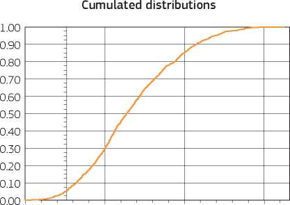
-26,000,000 24,000,000 74,000,000 124,000,000
ENPV
Punctual probability
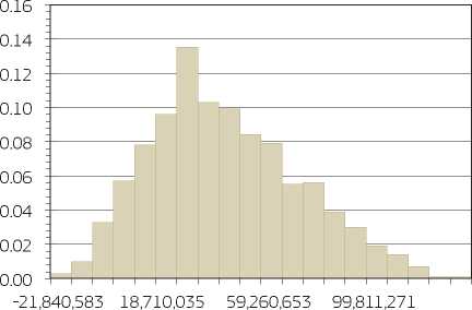
ENPV
Source: Authors
The cumulated probability curve (or a table of values) assesses the project risk, for example verifying whether the cumulative probability for a given value of NPV or IRR is higher or lower than a reference value that is considered to be critical. In the example shown in the above figure, the cumulative probability of an ENPV value of EUR 18,824,851, which is set at 50 % of the base value, is 0.225, a value high enough to recommend taking preventive and mitigation measures against the project risk. For a more detailed illustration of how to perform a probabilistic risk analysis and how results should be interpreted see Annex VIII.
The implementation of the steps described above defines the risk prevention and mitigation strategy of the project. Generally, a neutral attitude towards risks is recommended because the public sector might be able to pool the risks of a large number of projects. In such cases, the assessment of the switching values and of the scenario analysis results, followed by a well-established risk matrix (plus, a probabilistic risk analysis if necessary) will summarise the risk assessment. In some cases, however, the evaluator or the project promoter can deviate from neutrality and prefer to risk more (risk-taker) or less (risk-adverse) for the expected rate of return. However, there must be a clear justification for this choice.
Risk assessment should be the basis for risk management, which is the identification of strategies to reduce risks, including how to allocate them to the parties involved and which risks to transfer to professional risk management institutions such as insurance companies. Risk management is a complex function, requiring a variety of competences and resources, and it can be considered as a role for professionals, under the responsibility of the managing authority and the beneficiary. The project promoter should, however, following the risk assessment, at least identify specific measures (including responsibilities for their application) for the mitigation and/or prevention of the identified risks, according to international good practice. For a more detailed discussion about the assessment of acceptable risk levels and the definition of risk prevention and mitigation strategies see Annex VIII.
✓ The sensitivity analysis is extended to all the independent variables of the project and, among them, the critical variables are identified.
✓ A large enough numerical scale (i.e. a scale of 1-5) is used for adequate differentiation of probability of occurrence and impact levels of the adverse effects.
✓ The cost of prevention/mitigation measures is included within the investment and/or O&M costs. This includes risks linked to natural disasters or other similarly unforeseeable events which need to be either covered in the technical design of the project and/or adequately insured (if possible).
✓ The switching values for critical variables are calculated also when projects show a negative FNPV(K) after EU assistance. The necessary variation of a key variable to reach the benchmark is valuable information for the appraiser.
✓ If, after all prevention/mitigation measures, there is still a considerable risk in the project, a probabilistic analysis is carried out in addition to the qualitative assessment to quantify the probability of risk occurrence.
✓ Probability distributions of the input variables are adequately determined, for example on the basis of collected experience in past projects.
X Risks that are out of the control of the project promoter or other stakeholders (i.e. change of legislation) are neglected in the analysis, although they may substantially contribute to the success/failure of the project.
X Too aggregated variables (e. g. benefits as a whole) are taken into account in the sensitivity and risk analysis. As a consequence, it is not possible to identify which parameters the prevention/mitigation measures have focused on.
X Independently from the type of analysis, risk prevention/mitigation measures are not identified.
X A too generic discussion on risk causes and prevention measures is carried out with no mention of their likelihood of occurrence and/or identification of impacts.
X There is no identification of the risk ‘manager’, i.e. the function responsible for the implementation of the identified risk prevention/mitigation measures.
Table 2.16 Risk prevention matrix. Example
|
Adverse event |
Variable |
Causes |
Effect |
Timing |
Effect on cash flows |
Probability (P) |
Severity (S) |
Risk Level |
Prevention and/or Mitigation measures |
Residual risk |
|
Construction delays |
Investment cost |
Low contractor capacity |
Delay in service starting |
Medium |
Delay in establishing a positive cash flow including benefits materialisation |
C |
III |
Moderate |
Set up of a Project Implementation Unit to be assisted by technical assistance for project management during implementation. |
Low |
|
Project cost overrun |
Investment cost |
Inadequate design cost estimates |
Investment costs higher than expected |
Short |
Higher (social) costs in the first phase of the project |
D |
V |
Very high |
The design of the project must be revised. |
Moderate |
|
Landslides |
Not applicable |
Inadequate site investigation |
Interruption of the service |
Long |
Extra costs to rehabilitate the service |
A |
III |
Low |
Close monitoring |
Low |
|
Delayed obtainment of permits |
Not applicable |
Low political commitment; Mismanagement of the licensing procedures process |
Delay in commencement of works |
Short |
Delay in establishing a positive cash flow including benefits materialisation |
A |
II |
Low |
Close monitoring |
Low |
|
Public opposition |
Not applicable |
Inadequate market strategy Underestimation of threats |
Demand lower than expected |
Medium |
Lower revenues and social benefits |
C |
V |
High |
Early definition of an appropriate social plan; Awareness-raising activities and campaigns to raise the level of social acceptance |
Moderate |
Source: Authors
GUIDE TO COST-BENEFIT ANALYSIS OF INVESTMENT PROJECTS
The following checklist closes the chapter. It is intended as a suggested agenda both from the standpoint of the project promoter, who is involved in preparing the project dossier, and from that of the project examiner, who is involved in reviewing the quality of the appraisal.
|
Step |
Question |
|
General |
• Has an incremental approach been adopted? • Is the counterfactual scenario credible? • Has an appropriate time horizon been selected? • Have project effects been identified and monetised? • Have appropriate financial and social discount rates been adopted? • Does the economic analysis build on the financial analysis? • Is the methodology adopted consistent with the Commission’s or Member States’ own guidance? |
|
Presentation of the context |
• Is the social, institutional and economic context clearly described? • Have all the most important socio-economic effects of the project been considered in the context of the region, sector or country concerned? • Are these effects actually attainable given the context? • Are there any major potential constraints to project implementation? |
|
Definition of objectives |
• Does the project have clearly defined objectives stemming from a clear assessment of the needs? • Is the project relevant in light of the needs? • Are the project objectives quantitatively identified by means of indicators and target values? • Is the project coherent with the objectives of the Funds and the EU operational programmes? • Is the project coherent with the national and regional strategies and priorities, as defined in their development plans? • Are the means of measuring the attainment of objectives and their relationship, if any, with the targets of the operational programmes indicated? |
|
Identification of the project |
• Does the project constitute a clearly identified self-sufficient unit of analysis? • Have combinations of self-standing components been appraised independently? • Has the technical, financial and institutional capacity of the promoter been analysed? • Has the impact area been identified? • Have the final beneficiaries eventually profiting from the project been identified? • If the project is implemented by a PPP, is the PPP arrangement well described, are the public and private parties clearly identified? • Whose costs and benefits are going to be considered in the economic welfare calculation? • Are all the potentially affected parties considered? |
|
Technical feasibility and environmental sustainability |
• Has current demand for services been analysed? • Has future demand for services been forecasted? • Are the demand forecasting method and assumptions appropriate? • Does the application dossier contain sufficient evidence of the project’s feasibility (from a technical point of view)? • Has the applicant demonstrated that other alternative feasible options have been adequately considered? • On what criteria was the project optimal option selected? Are these criteria appropriate for the type of project? • Is cost of measures taken for correcting negative environmental impacts included in the cash flows considered in the CBA? • Is the technical design appropriate to the achievement of the objectives? • Is capacity utilisation rate in line with demand expectations? • Are the project cost estimates (investment and O&M) adequately explained and sufficiently disaggregated to allow for their assessment? |
|
Step |
Question |
|
Financial analysis |
• Have depreciation, reserves, and other accounting items which do not correspond to actual cash flows been excluded from the analysis? • Has the residual value of the investment been properly calculated and included in the analysis? • In the case of using current prices, has a nominal financial discount rate been adopted? • Has VAT, if recoverable by the beneficiary, been excluded from the analysis? • Have transfers and subsides been excluded from the computation of the project revenues? • If tariffs are levied from users, how has the polluter-pays-principle been applied, what is their cost recovery level in the short, medium and long-term? • If an affordability cap is applied to tariffs, has an affordability analysis been carried out? • Is the financial sustainability analysed at project and, where appropriate, operator level? • If the project is not financially sustainable by itself (produces negative cash-flows at some point), is it explained how the required funds will be ensured? • Have the main financial performance indicators been calculated (FNPV(C), FRR(C), FNPV(K), FRR(K)) considering the right cash-flow categories? • If private partners are involved, do they earn normal profits as compared with financial benchmarks in the sector? |
|
Economic analysis |
• In the case of market distortions, have shadow prices been used to better reflect the social opportunity cost of the resources consumed? • Is the Standard Conversion Factor calculated and applied to all minor non-traded items? • In the case of major non-traded items, have sector-specific conversion factors been applied? • Has the appropriate shadow wage been chosen for the labour market? • If cash-flows present fiscal requirements, have market prices been corrected? • Have non-market impacts been considered for the evaluation of the project economic performance? • Have externalities been included in the analysis, including climate change effects? • Are the unit values for quantification of economic benefits and externalities and their real growth over time adequately presented/explained? • Have the main economic performance indicators been calculated (ENPV, ERR and B/C ratio) considering the right categories of cost and benefits? Is there any risk of benefit double counting? • Is the economic net present value positive? If not, are there important non-monetised benefits to be considered? |
|
Risk assessment |
• Is the sensitivity analysis carried out variable by variable and possibly using switching values? • Has the scenario analysis been carried out? • What is the proposed risk prevention and mitigation strategy? • Has a full risk prevention matrix been built? • Have risk mitigation or prevention measures been identified? • If the project appears to be still exposed to risk, has a probabilistic risk analysis been carried out? • What is the overall assessment about the project risk? |
The EU transport infrastructure strategy, as defined in the TEN-T74 Guidelines, focuses on improving transport infrastructure quality through new investment and the efficient use of pre-existing infrastructure in order to improve accessibility, mobility and safety, as well as to match transport demand. Related investments priorities are defined under the thematic objective 7 ‘Promoting sustainable transport and removing bottlenecks in key network infrastructures', which focuses on:
• supporting a multimodal Single European Transport Area by investing in the trans-European transport network (TEN-T) network (investment priority 7a);
• enhancing regional mobility through connecting secondary and tertiary nodes to TEN-T infrastructure (7b);
• developing and improving environmentally-friendly and low-carbon transport systems, including inland-waterways and maritime transport, ports and multimodal links, and promoting sustainable regional and local mobility75 (7c);
• developing and rehabilitating a comprehensive, high quality and interoperable railway system (7d).
According to the Common Strategic Framework, actions financed under the ERDF and the Cohesion Fund in the transport field shall be planned in close cooperation with the Connecting Europe Facility (CEF), which is a directly managed fund created in 2012 for accelerating cross-border investments in the field of trans-European networks, maximising the synergies between transport, energy and telecommunications policies, and ensuring funding from both the public and private sectors.
The CEF will concentrate on projects with a high EU added value, in particular in the core network for cross-border infrastructure (as pre-identified in the Annex of the CEF Regulation) and for railway, while the Cohesion Fund and the ERDF will concentrate on high EU added-value projects to remove bottlenecks in transport networks by supporting TEN-T infrastructure, for both the core and the comprehensive network.
In addition, transport investments must be closely linked to the needs identified in national transport plans (cf. thematic ex-ante conditionality 7.1), based on a rigorous assessment of transport demand (both for passengers and for freight). These plans should identify missing links and bottlenecks and should set out a realistic and mature pipeline for projects envisaged for support from the ERDF and Cohesion Fund. The aim is to ensure a better interoperable integration between transport modes and a stronger focus towards the Trans-European Networks in 2020 and beyond.
As illustrated in the box below, EU policies and interventions have mainly focused on: development of the infrastructure network; regulation and competition among and between modes intended to open up the national markets and make transport services more competitive and interoperable at the EU level; setting prices correctly (including charging for infrastructure use and internalisation of external costs); and providing safe infrastructure and/or improving safety conditions.
White Paper on Transport (March 2011)
Proposal from the Commission for a European Parliament and Council regulation on Union guidelines for the development of the trans-European transport network (COM/2011/0650)
Roadmap to a Single European Transport Area -Towards a competitive and resource efficient transport system - White Paper (COM/2011/144)
Keep Europe moving - Sustainable mobility for our continent, Mid-term review of the European Commission’s 2001 Transport - White Paper (COM/2006/314)
European transport policy for 2010: Time to decide - White Paper ( COM/2001/370)
Roadmap to a Single European Transport Area: Facts and figures Urban public transport policy Connecting Europe Facility
European Commission 2014, Building the Transport Core Network: Core Network Corridors and Connecting Europe Facility, COM(2013) 940 final
European Commission, 2013, The Fourth Railway Package - Completing the Single European Railway Area to Foster European Competitiveness and Growth
European Commission, 2011, Regulation of the European Parliament and the Council establishing the Connecting Europe facility
TEN-T: A policy review - ‘Towards a better integrated trans-European transport network at the service of the common transport policy’, Green Paper
Decision 661/2010/EU of the European Parliament and the Council of 7 July 2010 on Union guidelines for the development of the trans-European transport network
Trans-European Networks: Towards an integrated approach, COM/2007/0135
European Commission, 2007, Regulation of the European Parliament and the Council N. 1370 on public passenger transport services by rail and by road
Road Tolling Directive 2004/52/EC and Decision 2009/750/EC
Directive 2006/38/EC ‘Euro-vignette’ amending Directive 1999/62/EC on the charging of heavy goods vehicles for the use of certain infrastructures (see following box)
Directive 2004/49/EC amending Directive 2001/14/EC on the allocation of railway infrastructure capacity and the levying of charges for the use of railway infrastructure and safety certification
Directive 2011/76/EU amending Directive 1999/62/EC on the charging of heavy goods vehicles for the use of certain infrastructures
Directive 2008/57/EC of the European Parliament and the Council of 17 June 2008 on the interoperability of the rail system within the Community: OJ L 191/1 of 18 July 2008
Commission Decision of 25 January 2012 on the technical specification for interoperability relating to the control-command and signalling subsystems of the trans-European rail system
The objectives of a transport project, namely the specific functions the infrastructure has to perform, must be consistent with the territorial context of the region or country (or cross-border area) where the project is built. As a minimum, the following information should be presented in order to outline the baseline elements.
Table 3.1 Presentation of the context. Transport sector
|
Assumptions | |
|
Socio-economic trend |
- National and regional GDP growth - Demographic change - Industrial and logistics structure and developments (freight transport) - Forecasts in employment - Forecast in indices of specific economic sectors in which the area covered by the infrastructure is suited (e.g. value added growth in tourism) |
|
Political, Institutional and Regulatory |
- Reference to EU directives and sector policy documents - Reference to the long-term national, regional and local planning documents and strategies, including, for example, the General Transport Development Plan and the Public Transport Development Plan - Reference to the priority axis and the intervention areas of the OP - Any pre-existing planning authorisations and decisions |
|
Existing service conditions |
- Detailed information about the existing transport infrastructure in the area - Information about competition from alternative transport modes - Planned and/or recently executed investments that may affect the project performance - Information about historic and present traffic patterns - Statistics in motorisation, mobility and accessibility of the area - Technical characteristics of the service currently provided - Service quality, frequency and safety - Infrastructure capacity |
Source: Authors
The next step is to clearly state the main objectives of the transport project. These are generally related to the improvement in travel conditions for goods and passengers both inside the impact area and to and from the impact area (accessibility), as well as improvements in both the quality of the environment and the wellbeing of the population served. In more detail, projects will typically deal with the following objectives:
• reduction of congestion within a network, link or node by resolving capacity constraints;
• improvement of the capacity and/or performance of a network, link or node by increasing travel speeds and by reducing operating costs and accidents;
• improvement of the reliability and safety of a network, link or node;
• minimisation of GHG emissions, pollution and limitation of the environmental impact (important examples are projects supporting the shift from individual, i.e. cars, to collective transport);
• adjustment to EU standards and completion of missing links or poorly linked networks: transport networks have often been created on a national and/or regional basis, which may no longer meet the transport requirements of the single market (this is mainly the case with railways);
• improvement of accessibility in peripheral areas or regions.
Objectives must be aligned with the priorities identified in the OP and Transport Master Plan/Strategy in the context of ex ante conditionality. When feasible, they should be quantified and targeted with the use of indicators, logically linked to the project benefits (see section 3.7). For example, indicators including expected traffic volumes, travel times, average speeds, etc., can be used to show the link between the materialisation of the project benefits and the achievement of the stated objectives.
A good starting point for briefly, but clearly, identifying the infrastructure is to state its functions, which should be coherent with the investment objectives. This should be followed by a description of the project typology, that is whether it is a completely new facility, or a link to a larger infrastructure, or an extension/upgrade of a pre-existing one77 (see box). Finally, a detailed list of the physical realisations must be included.
New infrastructures to satisfy increasing transport demand Completion of existing networks (missing links)
Extension/renovation of existing infrastructures Investment in safety measures on existing links or networks
Improved use of the existing networks (i.e. better use of under-utilised network capacity) Improvement in inter-modality (e.g. interchange nodes)
Improvement in networks interoperability
Improvement in the management of the infrastructure investment
The identification of the project as a self-sufficient unit of analysis is usually a challenging issue in the transport sector. This is because most transport projects belong to a wider network and any investment decisions and implementation are not isolated, but are part of a larger system of public interventions, as well as the need to be physically integrated with other complementary infrastructures. In project identification, the basic principle is that its scope must always be a stand-alone socio-economic and technical unit: i.e. it should generally be functional and independently useful from a transport perspective without depending on the construction of other projects (which may however provide synergies). That considered, the following basic rules can be applied (see also section 2.6):
• when the project consists of realising a given section, sub-portion or phase of a well identified transport investment, the CBA (and the supporting feasibility study) should be focused on the entire investment, regardless of the object of the EDRF/Cohesion Fund assistance;
• when the project contributes to implementing a larger investment strategy or plan, encompassing a set of interventions all aimed at achieving the same priority, each intervention should undergo a CBA. For example, a project may consist of the completion of a trans-national link under the TEN-T. Here, the economic appraisal should not focus on the entire link, but only on the project's section where different options are available.
For example, the construction of a third lane for a two-lane motorway, the laying of a second track or the electrification and automation of an existing rail line.
When developing a demand analysis for transport investments, particular attention should be paid to the sensitivity of traffic to some critical variables such as:
• demographic changes, including, amongst others, the number of people split into age structure, level of education and number of people of productive and non-productive age;
• socio-economic changes, including, amongst others, GDP level in analysed area, incomes, level of unemployment, economic structure of regions being served currently or in the future by the transport infrastructure;
• industrial and logistics structure and developments: location of concentrated industrial activities, natural resources, main transport hubs (ports and airports), logistics structure, and expected developments in supply chain organisation (clustering, unitisation, change in distribution patterns);
• elasticity with respect to quality, time and price (see box): travel demand characteristics, structure and elasticity are particularly important in those projects related to charged infrastructures, since the expected traffic volumes are determined by fare levels and the transport conditions;
• capacity constraints on competing modes and strategies in place, for example in terms of investments foreseen. This point is particularly relevant for long term investments: in the time span required to complete the intervention, the traffic that may be potentially acquired by the new infrastructure may shift to other modes and, if so, then it may be difficult to move it back.
• spatial changes leading to changes in the distribution of traffic potential;
• change of traffic management policies, e.g. existence of constraints in using the car in determined areas (this is particularly the case of urban public transport) or establishment of taxes or subsidies for competing modes;
• technological changes impacting the cost structure for the project and its alternatives through changes in e.g. fuel efficiency, fleet composition or productivity.
Given the uncertainty of the future trends of these variables, it is generally recommended to develop, as a minimum, three traffic scenarios (high, most likely and low), which should further feed into risk analysis. These should be based on different developments of both exogenous (e.g. GDP growth) and endogenous (e.g. pricing policy) variables. Demand forecasting should be completed for the scenario without-the-project, and for each project option (see below).
Fares, tolls and other pricing policies will influence the expected volume of demand and the distribution of demand across transport modes. It is therefore important, whenever a different pricing hypothesis is introduced, to reconsider the demand estimates and allocate the correct traffic volumes to each mode. With regard to pricing criteria, it is important to distinguish between:
- fares which maximise the proceeds for the managers/constructors of infrastructures: these kinds of fares maximise the capacity for self-financing;
- efficiency fares: these take into consideration the social surplus and also consider the external costs (congestion as well as the environmental and safety costs).
Efficient pricing should, in principle, be based on social marginal costs and requires the ‘internalisation of external costs’ (polluter pays principle), including congestion and environment costs. Social efficiency requires that users pay both the marginal private or internal and external costs that they impose on society. An efficient structure of charges confronts users with the marginal social costs of their decisions.
In order to develop traffic forecasting, some justified specific assumptions should be adopted with regard to:
• the project’s impact area, in order to limit the traffic study and the related economic impacts. It is important to identify the demand without the project and the impact of the new infrastructure, as well as identify other transport modes potentially involved;
• the degree of complementarity and competition among transport modes. In particular, competing modes and alternative routes, fares and costs for users, pricing and regulation policies, congestion and capacity constraints and expected new investments should be assessed;
• the deviations from past trends, including changes in tax regime, energy prices or toll collection policy;
• the relative sensitivity of demand patterns (such as modal share or volume of traffic) to changes in the transport supply.
Traffic modelling78 is usually required for demand analysis, which enables the simulation of traffic distribution on the network thereby providing indication of how trips will respond, over time, to changes in transport supply and demand. Trip developments may be the consequence of changes in the demand for transport and/or in the transport network itself (i.e. the building of new transport infrastructure and/or provision of operated services).
Different models exist, ranging from the development of relatively simple spreadsheet models79 (which are generally bespoke and constructed by users for a particular calculation) to network models that describe a defined impact area and are generally more complex since they can involve ‘feedback loops', where the resulting state of the network can impact on user decisions. These complex models incorporate significant volumes of information on the demand structure, the transport network and its dynamics (e.g. timetables, interconnections, etc.) to describe large numbers of transport movements over a specified period. Data is typically coded in the form of attributes for each transport link in the network, including speed, quality, and the travel modes that use each link.
The choice of the appropriate model depends on a large number of factors, including the nature of the options to be tested, geographical location, scope, size and likely key impacts so that is not liable to adopt a ‘one size fits all' approach to developing transport models in order to assess this range of issues. In general, the larger the project framework complexity, the higher the need for more sophisticated and complex models. Complex transport modelling is considered compulsory in large projects, e.g. if its size can significantly influence other traffic services or regional transport pattern.
Although there is currently no detailed guidance at EU level for the development and application of transport models, basic principles and features of modelling can be derived from national guidance, which the project promoter should always refer to. These include:
• traffic modelling is used to predict the travel choice made by users travelling through the network, and to load the resulting trip movements to the modelled network based on a selection of the most likely routing for each trip. The model then describes the loaded transport network after this process has been completed;
• the state of the transport network in future years on the basis of growth in travel demand, committed network changes and changes in socio-economic data can also be defined. Future years usually coincide at least with the opening year and a distant forecast year which is used for assessment of long-term capacity needs or is the end year of economic evaluation;
• many transport models require substantial input data derived from standard statistics and special surveys for building a model of trips, a model of the network and for understanding current traffic flows and demand structure for the purpose of model calibration. This is essential for the model to be sufficiently accurate and have credibility for planning and decision making;
• the output from the transport model is used to design adequate sizing and features of the investment, to verify the appropriateness of planned infrastructure capacity, and provides quantitative information that informs the scheme design, the CBA and the EIA. 76 77
Whatever model and modelling process is adopted, all hypotheses and assumptions applied to estimated existing and future demand should be made explicit by the project promoter. Although the analysis of the input data for traffic modelling is not a task of the CBA, nevertheless, there should be the source should be given of all quoted demographic, spatial and economic data.
Taking into account the requirements for economic analysis, traffic forecast outputs are developed for passenger and/or cargo traffic. Outputs shall include all information necessary for further technical analyses as well as financial and economic analyses. Although each subsector has its own indicators of traffic forecasts, the following demand parameters are usually collected to feed the CBA model:
• number of vehicles (cars, trains, buses, airplanes, ships, etc.) in absolute value, per unit of time (e.g. Annual Average Daily Traffic (AADT), trains per day, etc.) and/or per average trip length (e.g. vehicles-km, trains-km, etc.);
• number of vehicles broken down by category, speed class and road category;
• number of passengers, passenger-hours and passenger-km78;
• cargo traffic in tons, ton-hour and ton-km;
• travel times and other network performance indicators.
Types of traffic response
Traffic types can be divided according to their behavioural response to a project. This qualification will become relevant when it comes to the assessment of the socio-economic impacts of the project. The classification proposed in this guide is as follows79:
• existing traffic: current traffic on the network of reference (new projects) or on the infrastructure to be upgraded/ reconstructed;
• diverted traffic: traffic which is attracted to the project from other routes or transport modes;
• generated/induced traffic: additional traffic flows that result from a transportation infrastructure improvement due to new users attracted by better conditions of transport80.
Depending on the traffic system perspective, and on the actual availability of data on generalised costs from the traffic model, the assessment of socio-economic benefits for each of these categories can be performed differently (see section 3.8 below).81
Also, for the purpose of the economic assessment, the traffic surveys should also provide information on the share of trips by travel purpose, for instance business, commuting and leisure trips. An additional distinction by short and long distance trips can be relevant for road and railways trips.
The project should be identified after the assessment of all promising strategic and technical alternatives on the basis of physical circumstances and available technologies. The main potential for distorting the evaluation is the risk of neglecting relevant alternatives, in particular low-cost solutions, such as managing and pricing solutions, infrastructure interventions that are considered as not ‘decisive' by designers and promoters, etc.
Possible design options in transport include: i) mode; ii) location/route; iii) alignment, iv) technical solutions; v) interchanges; etc. Different options may have different demand, costs and impacts.
Options might include synergies in co-deployment of transport and NGA infrastructure, in line with the Directive 2014/61/ EU, in view of smartening the transport systems, improving efficiency in the use of public funds, and significantly increasing the socio-economic impact of projects.
For option selection, the suggested approach is generally to use Multi-Criteria Analysis for shortlisting the alternatives, then CBA to compare the results of the shortlisted options and consequently select the most promising one. It is worth stressing that option analysis should be developed standardly in concept stage feasibility studies prior to design and funding application preparation. In this case, the promoter should properly describe the options analysis in the feasibility study, in order to demonstrate that the available options have been subject to a robust assessment and that the selected option was the best from a socio-economic perspective. Otherwise, if the appropriate analysis was not formerly completed, it would then form part of the feasibility study, which is an annex to the project application.
Finally, option analysis can also be used later to review the efficiency of previous designs, especially when socio-economic circumstances have changed. This can lead to project re-design.
Investment costs disaggregation is project-specific, although the transport sub-sectors are usually characterised by common cost categories for both initial investment and renewals82. For an illustrative list of investment outlays in the road and railway sectors, see the case studies at the end of the chapter. As general remarks valid for any transport investment, the following can be highlighted:
• estimates must be based on appropriate benchmarks with projects of comparable characteristics, based on best available technologies, etc.;
• it is recommended to present both the total cost of the project and the unit value (e.g. cost per km, cost per unit of rolling stock, etc.);
• costly engineering structures (tunnels, bridges, overpasses, etc.) should always be shown separately in a cost statement to allow for benchmarking;
• it is necessary to ensure that the project will include all the works required for its functioning (for example, links to the existing networks, technological plants, stations with related services, urban renewal works adjacent to public transport investments, etc.);
• cost of land83 and costs for environmental protection, including e.g. noise barriers and other noise protection, drainage, greenery, animal passages, etc., and/or for the integration of the works in the territory (e.g. for the preservation of the landscape integrity, etc.) are usually main items to be included in the investment costs.
In the transport sector, O&M costs can be generally grouped into the following categories:
• infrastructure operations, e.g. repairs, current maintenance, materials, energy, Traffic Management System;
• services operations, e.g. staff cost, traffic management expenses, energy consumption, materials, consumables, rolling stocks maintenance, insurance, etc.;
• services management, e.g. services management itself, fare/tolls collection, company overheads, buildings, administration, etc.
As for the timing of the expenditure, O&M costs should cover (and is usually distinguished in):
• routine maintenance: yearly work required to keep the infrastructure technically safe and ready for day to day operation as well as to prevent deterioration of the infrastructure assets;
• periodic maintenance: all activities intended to restore the original condition of the infrastructure.
In financial analysis, O&M costs should be estimated in both the with and without project scenarios. Significant difference may, however, exist between the two scenarios, especially when maintenance and repair have been neglected in the past. For the estimation of O&M costs in the counterfactual scenario, in particular, periodic and routine maintenance costs should correspond to reaching the target without the project standard of operations with minimal investments. All assumptions taken should be carefully documented in the project dossier.
Financial inflows will be represented by the proceeds from the charges applied to users for the access to the infrastructure or the sale of transport services, or related to sale or rent of land or buildings. The estimate for the proceeds must be consistent with the demand elasticity and trends of explanatory variables and, in a more general sense, with traffic modelling output.
The estimation of revenues should be based on the following elements:
• traffic volume forecast (changes of passenger and cargo traffic);
• projection of changes in charge system and pricing policy;
• traffic forecast for each projection of charge system;
• subsidy/compensation projection.
An indicative list of typical revenues to be considered for calculation of the financial profitability is provided in the table below.
Table 3.2 Typical sources of revenue by transport mode
|
Revenues from transport activities |
Revenues from non-transport activities | |
|
Road |
Tolls and/or other users charges |
Value of scrap material Rental of service stations Advertisement on service stations |
|
Railway |
Access charges to railway line |
Advertisement on trains and/or in railway stations |
|
(in the case of infrastructure projects) Tickets (in the case of roiling stock projects) |
Commercial premises in railway stations | |
|
Urban |
Tickets and subscriptions |
Commercial premises in stations |
|
transport |
Advertisement on vehicles and/or on stations or bus stops | |
|
Airports |
Take-off or landing charge |
Commercial services |
|
Passenger charge |
Real estate rental | |
|
Parking charge |
Food services | |
|
Cargo charge |
Transport services Advertising services Car parks | |
|
Seaports |
Basin, berth dues, etc. |
Commercial premises |
|
and inland waterways |
Tariff for inland cargo ship |
Logistics Advertising on vessels |
|
Intermodal |
Access charges to railway line |
Commercial premises |
|
facilities |
Tariff/fee for cargo storage and transhipment |
Logistics |
Source: Authors
If the situation on a given transport service is such that revenues from transport and non-transport activities do not fully cover the cost of operation, the gap must be filled with other sources to avoid the closure of the service. This usually implies that an operating subsidy or compensation is provided from public funds. Under such circumstances, this type of inflow must be separated from the overall revenue projection because, as highlighted in chapter 2, they do not concur for the calculation of the EU contribution and the financial performance indicators (but they count for sustainability).
As a result of the revenue analysis, the projection of the total revenues for the entire time horizon of the analysis should be prepared in both with and without-the-project scenarios.
As mentioned in chapter 2, it is recommended to carry out the financial analysis at a consolidated (owner + operator) level. This is particularly feasible when there is only one operator, which provides the transport service on behalf of the owner, usually by means of a concession contract. This is often the case of road and urban transport services.
In other cases, on the contrary, the consolidation of the analysis cannot be feasible. In liberalised markets, the number of operators can be very large, e.g. in airports but, to some extent, also in seaports and railways. Given the high number of data that would be required, together with legal and information protection issues, the financial analysis of these investments is more frequently carried out from the viewpoint of the infrastructure owner. In such a case, the revenues to be accounted for in the CBA are those originating from the operators or from third parties (e.g. tenants of commercial spaces, etc.) to the owner for the use of the infrastructure (usually access charges, see below). Conversely, in the case of projects implemented by operators (e.g. rolling stock renovation in urban transport), the revenues are those originating from the sale of the service to final users, as well as any other operating revenues accruing to the operator for the use of the infrastructure by third parties.
In transport projects the main direct benefits are measured by the change of the following measurable.
• The consumer surplus, defined as the excess of users' willingness-to-pay over the prevailing generalised cost of transport for a specific trip. The generalised cost of transport expresses the overall inconvenience to the user of travelling between a particular origin (i) and destination (j) using a specific mode of transport. In practice, it is usually computed as the sum of monetary costs borne (e.g. tariff, toll, fuel, etc.) plus the value of the travel time (and/or travel time equivalents, such as the inconvenience of long intervals) calculated in equivalent monetary units. Any reduction of the generalised cost of transport for the movement of goods and people determines an increase in the consumer surplus. The main items to be considered for the estimation of the consumer surplus are:
- fares paid by users;
- travel time;
- road users Vehicle Operating Costs.
• The producer surplus, defined as the revenues accrued by the producer (i.e. owner and operators together) minus the costs borne. The change in the producer surplus is calculated as the difference between the change in the producer revenue (e.g. rail ticket income increase) less the change in the producer costs (e.g. train operating costs increase). This might be particularly relevant for public transport projects or toll road projects, especially if the project is expected to feature significant traffic (generated or induced) or a substantial change in fares. The main items to be considered for the estimation of the consumer surplus are:
- fares paid by users (and received by the producer); and
- producer operating costs.
It must be noted that fares paid by users for the use of the infrastructure appear in the economic analysis as a cost to the user in the estimation of the consumer surplus and as a revenue to the producer in the estimation of the producer surplus. Thus, for existing traffic (see section 5.5.3 above for definitions), this implies that fares are always cancelled out in the analysis. However, this is never the case for the calculation of benefits to generated/induced traffic, which are generally approximated via the Rule of Half (see box), and would also not apply in the cases where the benefits to the diverted traffic are also estimated via the Rule of Half (see section 3.8.1). In such cases, the producer revenues and associated user charge costs will not be cancelled out.84
This implies that the economic analysis of transport projects can be structured differently depending on two main situations:
• in cases where the project is not expected to change traffic volumes, there is no need to estimate the changes of the consumer and producer surplus because the fares paid by users will always be cancelled out. A simplified approach can therefore be adopted and the analysis will just rely on the estimation of the net effects on users, in terms of travel time savings and, for road projects, Vehicle Operating Cost savings85. The case study on road investment, at the end of this chapter, provides an example of this approach;
• in cases where the project is expected to change traffic volumes or when transport pricing strategies are introduced or expected to be changed, the fares paid by users will not be cancelled out. The analysis will therefore consist of estimating the net impacts on both the consumer and producer surplus. This implies that fares need to be separately accounted for, as well as all the changes in the producer operating costs (if not already captured in the financial analysis - as it happens when the analysis is not consolidated). The case study on rail investment provides an example of this approach.
In addition, any transport project may generate relevant non-market impacts on safety and the environment that always need to be evaluated.
Table 3.3 reviews the main effects and the relative evaluation methods to be considered for the economic appraisal of transport infrastructure projects. Fares are not included since they have already been discussed in section 3.7.3.
Table 3.3 Typical economic benefits (costs) of transport project
|
Effect |
Valuation method |
|
Travel time savings |
- Stated preferences - Revealed preferences (multi-purpose household/business surveys) - Cost saving approach |
|
Vehicle Operating Costs savings |
- Market value |
|
Operating costs of carriers |
- Market value |
|
Accidents savings |
- Stated preferences - Revealed preferences (hedonic wage method) - Human capital approach |
|
Variation in noise emissions |
- WTP//WTA compensation - Hedonic price method |
|
Variation in air pollution |
- Shadow price of air pollutants |
|
Variation in GHG emissions |
- Shadow price of GHG emissions |
Source: Authors
In what follows, the main information needed and the practical instructions to evaluate the benefits (costs) illustrated above are presented. It is worth noting that economic effects other than those listed in table 5.3 can be generated. This pertains mainly to the wider impact on regional development, which is frequently associated with large transport investments. For instance, the improvement of an airport can influence socio-economic growth by activating the job market, developing local businesses, increasing community activity and boosting tourism.
As previously mentioned, the approach of the Guide is to exclude indirect and wider impacts from the CBA (see section 2.9.11). It is recommended, however, to provide a qualitative description of these wider impacts on secondary markets, public funds, employment, GDP, etc. in order to better explain the contribution of the project to the EU regional policy goals.
The Rule of Half (RoH) relies on the consideration that, without the project, non-travelling users Willingness To Pay (WTP) is lower than the (prior) generalised cost of transport. After project implementation the (new) generalised cost of transport is lowered so that some previously non-travelling people decide to travel.
Although the absolute WTP is not known, the average change in consumer surplus of the generated traffic can be estimated as half of the difference between the original and the new generalised costs of transport on the improved mode for a given origin-destination (O-D) relation. It is half because a linear demand/cost graph is assumed where new users are spread evenly between two extremes: those requiring marginal motivation to start travelling (their WTP is already on the cusp between travelling and not travelling, so they get the full benefit of the change in generalised costs) and those requiring the full benefit of the change to the transport system to be motivated to travel (they get marginal net benefit). The RoH can be therefore expressed by the following formula:
gc = p+z+vz
where: p is the amount paid for the trip by the user (tariff, toll); z is the perceived operating costs for road vehicles (for public transport is equal to zero);r is the total time for the trip; v in the unit value of travel time.
Total consumer’s surplus (CS0) for a particular i and j in the Business As Usual (BAU) scenario is shown diagrammatically in the first figure. It is represented by the area beneath the demand curve and above the equilibrium generalised cost, area CS0.
User benefit = Consumer’s surplus^ - Consumer’s surplus^ where: 1 is the do-something scenario and 0 is the BAU scenario.
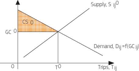
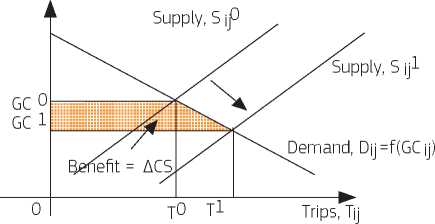
If there is an improvement in supply conditions the consumer’s surplus will increase by an amount of ACS, due to a reduction in equilibrium generalised cost and the total user benefit (for existing and new users) can be approximated by the following function, known as the rule of a half:
GCo i
ACS= JD(GC)dGC = Rule of one Half (RoH) = -(GCo - GCi)(To + Ti)
GCi 2
For the generated demand only (i.e. for new users), the benefits may be approximated by the following formula :
ACS(generated) = 1/2*(GC0-GC1)*(T1-T0)’
In the case of a totally new infrastructure, the RoH will not be directly applicable and the measurement of the benefits depends on the nature of the new mode, its placement in the mode hierarchy and transport network, and will often need to be derived from the users’ WTP or calculated with other approaches. For example see various integration and other methods suggested in World Bank Transport Note No. TRN-11 2005.
Source: Authors
Travel time saving is one of the most significant benefits that can arise from the construction of new, or improvement of, existing transport infrastructure.
Passengers traffic time savings
In carrying out CBA, different methods are possible to value time for passengers, whilst a distinction is usually made between the estimation of work and non-work travel time (including commuting).
The first method is to carry out specific empirical research and/or surveys in that country to estimate both work and non-work travel time. The approach consists of interviewing individuals using the stated preference method or conducting multi-purpose household/business surveys using the revealed preference method and then to estimate a discrete choice model on these data.
As a second option, value of time can be estimated adopting the cost saving approach88. The underlying logic is that time spent for work-related trips is a cost to the employer, who could have used the employee in an alternative productive way. The recommended process for valuing work time with the cost savings approach is as below.
• Establishing wage rates for a given country or region: the gross hourly labour cost (Euro per hour) must be derived from observed (or, in absence, from average national) wage rates. The main data source should be the national statistical office;
• Adjustment to reflect additional employee related costs: this would include paid holidays; employment taxes; other compulsory contributions (e.g. employer pension contributions) and an allowance for overheads required to keep someone employed. Social security payments and overheads paid by the employer shall therefore be computed and added to the estimated hourly labour cost.
The cost saving method is a simple approach to estimate a single value of work-time in a given country or region. This can, however, be enriched with further considerations and analysis, if necessary and feasible, as illustrated in the box below.
The preferred source from where to obtain value(s) of time at country level should be official national data, based on local research, provided that the methodology used is sound, robust and follows the general prescriptions illustrated above.89
For non-work travel time, the economic value of time savings is given by the difference between the marginal valuation of time associated with travelling and that associated with leisure. The implication is that there is no theoretical basis for deriving the economic value of non-work trips from the wage rate; instead the values have to be inferred from behaviour.
In the absence of national data using stated or revealed preference methods, the usual solution to this problem is to evaluate non-work travel time at a national average rate rather than at the rate the travellers appear to value their time themselves. In other words, non-work time can be assumed as a share of the work-related value. The review of the economic literature about value of time in specific countries suggests that non-working time usually ranges between 25 % and 40 % of the work time.90 86 87 88
- Labour market. The cost savings approach assumes that the gross wage rate in the labour market equals the marginal value product which the labour yields. However, this is not the case whenever distortions of the labour market exist. Thus, adjustments to reflect the level of unemployment in the country/region can be applied and the estimated value of time corrected by the shadow wage rate.
- Industrial sector. Under the cost savings approach the economic value of work time savings is the marginal productivity of the person making the saving; thus different workers will have different time valuations. Ideally, values of time (VOT) should be developed for each worker classification. However, for the economic appraisal to operate at this level of disaggregation also requires the demand forecasting to occur at the same level.
- Mode. Considering the relative qualities and comforts of one mode compared to the other modes (all other conditions being equivalent), value of travel time can be related to the mode of transport. For example, when considering average VOT associated with travellers using a certain transport mode, the average value of time of a bus traveller is usually lower than that of a car traveller. This is a characteristic of the fact that people with lower income will select slower and cheaper modes of transport (e.g. the bus) than richer people. Thus, it can be useful to differentiate the value of time by transport modes according to different people income level groups (where air and high speed rail transport are associated with higher income groups).
- Walking and waiting time. All other things being equal, an individual typically prefers travelling within a vehicle to spending time walking, waiting or transferring between services. This is borne out from evidence, as such the value of non-working time saved walking and waiting is higher than time saved whilst travelling within a vehicle. The exact magnitude of the difference between non-working in-vehicle time and walking and waiting time is dependent upon national cultures and characteristics. For example, Mackie et al (2003) have found within the UK walking time savings are valued at double in-vehicle time savings. Such variations may be explained by a range of cultural, racial and economic factors which drive personal preferences. In this regard, the World Bank recommends a weight of 1.5 for waiting and access time when national research is missing.
- Trip distance. The relationship between the value of (non-work) travel time and journey length includes increasing marginal disutility of travel time with journey length, greater significance of time constraints in longer distance journeys and differences in the trip purpose mix at long, relative to short distances. However, in practice it is expected that such situations will be rare so that a single value for travel time is used irrespective of trip distance. However, in cases where robust local or national specific data indicates that the values of non-work travel time savings increase with journey distance, data from revealed or stated travel behaviour can be used to adjust the value of time.
- Travel conditions. The comfort associated with travelling conditions, including the ability of the traveller to take advantage of the time spent travelling, also affects value of time. For example, VOT savings in congested car driving situations exhibit higher values than those in uncongested situations. This reflects both the value of reducing the variability of travel time and the unpleasantness of driving in congested conditions. In urban public transport, the availability of air conditioning, less crowded busses, etc. are very important to justify certain expenditures. Another critical aspect is the capacity to work during the trip, which is a key advantage of rail transport with regard to road and (short haul) air travel and explains the behaviour of many travellers.
Freight traffic time savings
Reduction in travel times will benefit freight traffic in the following ways:
• reduced driver (and any other persons necessarily travelling with the load,) wage costs per trip;
• reduced vehicle operating costs per trip;
• improved reliability, i.e. timely delivery of transported goods.
The valuation of the first benefit follows the same logic of passenger's traffic so that time savings for truck drivers (or rail carriers' crew members) is evaluated with the cost savings approach, whilst the valuation of the second is discussed below in section 3.8.2.
The last benefit item may arise through a number of mechanisms. If travel and transport times become more predictable, travellers and agents in freight transport would find it easier to arrive at the destination at the preferred moment and therefore reduce their safety margins in departure time. Also, in the case of perishables products, arriving at market earlier and in better condition thereby attract better prices; and reduced stockholding required through re-structuring of logistics and the supply sector. Its evaluation and inclusion within the economic benefits of a project is a complex issue which will require detailed case by case analysis. The following aspects should be taken into account when deciding whether to include time savings for freight:
• such analysis shall be considered only where large step changes in transport infrastructure are under consideration;
• benefit associated with reliability depends very much on the market segment in question as well as the time value of the commodity89;
• owing to specific conditions of the market, logistics chain and general service, benefits from time savings can be lost elsewhere. For instance, benefit from improved speeds is realised only if they are not lost in other parts of the logistics chain. The situation and risks should be analysed and demonstrated in any CBA. Key elements of the logistics chain influencing potential time losses are the priority given, and capacity available to, the type of freight traffic on the line, issues at transfer/marshalling/loading/unloading points and the administration at border points;
• care is needed to avoid double counting with vehicle operating costs savings calculations (for example distance reducing effects on operating costs should not be counted in travel time savings).
The methodology for the estimation of time value for freight should be based on the capital lock-up approach. This is based on the concept that value of time related to the movement of goods includes the interest costs on the capital invested in the goods during the time that the transport takes (important for high-value goods,), a reduction in the value of perishable goods during transit, but also the possibility that the production process is disrupted by missing inputs or that customers cannot be supplied due to lack of stock.
The valuation of the freight's value of time requires therefore an in-depth analysis of the MS's transport and logistic and supply sectors90. In a context of limited resources, it is suggested to refer to the economic literature where it is possible to find country-specific default values. The literature shows that reference unit values of time for freight vary significantly across countries: from over 1 EUR/tonne-hour to zero, and from small to large differentiation between commodities. For a review of the main studies and reports see the Bibliography section.
In this regard, HEATCO provides a framework with reference values for the EU-25. However, these values, particularly for rail freight, are relatively high as compared to other national-based studies because they include a full set of potential benefits (e.g. potential carrier company efficiency improvements). Thus, it is suggested to adopt them as a last resort and, in case, to include a scaling-down factor (e.g. low escalation elasticity against GDP).
In any case, the methodology used by the project promoter should be clearly presented, with all underlying assumptions and calculations made explicit. In general, since the values attributed to time are critical, the recommendation is to clearly report the VOT adopted and to check for consistency. In particular, MSs are encouraged to develop their own national guidance in order to propose unit reference VOT for both passengers and freight, provided that the methodology is complaint with the principles indicated in this guide.
The real value of work time is directly related to the real wage rate. Thus, it will grow with the projected wage rate, which is typically assumed to equal the growth in GDP per capita. The economic literature suggests escalating value of time for future years across the time horizon based on a default inter-temporal elasticity to GDP per capita growth of 0.7 to 1.0. This elasticity is expected to vary very little across market segments and to be stable over time. The value of non-work time is not related to the wage rate and as such there is no theoretical justification for linking it to wage rate growth. However, its value is related to income and any changes in income will affect that value. Studies in the UK91 and the Netherlands92 have indicated elasticity of value of time with respect to income of approximately 0.5 to 0.8.
It is generally recommended that value of both work and non-work time be treated as increasing over time in proportion to GDP per capita, unless there is local evidence to the contrary. For the sake of prudency, it is however recommended to use the lower elasticity values illustrated above: 0.7 and 0.5 for, respectively, work and non-work time. If HEATCO values are adopted as a last resort, the use of lower elasticity is recommended. In line with the use of constant prices, the inflation effect must not be taken into account for escalation.
Application rules
Once unit VOT are determined, benefit from time savings needs to be calculated separately, for:
• Already existing traffic of passengers and goods. For benefit calculation, the following procedure shall be adopted:
- take the forecast of existing traffic considering number of passengers/goods for each origin-destination (O-D) pair and for each year across the time horizon;
- take the travel time for each pair (O-D), on the basis of estimated average travel speed, for both with and without-the-project scenarios;
- split passenger traffic into motivations: work and non-work related trips93;
- calculate the time saving as the difference between travel time in the two scenarios;
- calculate the benefit for each traffic class using the unit values available.
• Passengers and goods diverted from other transport modes or routes. When calculating time costs for passengers diverted from other routes or means of transport, practice across Europe varies and yet there is no consensus on the correct approach to take. Several methods can be used reflecting different approaches followed in different countries. The treatment of diverted traffic would in particular depend on project-specific circumstances, including whether there is an increase in capacity, the degree of congestion that can occur as the infrastructure approaches full capacity, and the availability of alternative modes with sufficient capacity to accommodate traffic that cannot be accommodated in the without-the-project scenario. In this guide the following, simplified, approach is suggested:
- the Rule of Half should be applied to the travel cost change to the shifted mode whenever there is poor or no knowledge of the overall average generalised costs on O-D trips of either the transferred from, or transferred to, mode. Its application requires an estimate of mode shifted O-D movements;
- if there is good and sufficiently detailed and calibrated knowledge of average travel costs between origins and destinations on all considered modes, the full difference between travel costs on the switched to mode and switched from mode should be applied94. Time savings are thus calculated as the difference between the estimated travel speed in the with-the-project scenario and the travel speed in the alternative transport mode/route from which traffic is diverted;
- in the case of a totally new infrastructure, the Rule of Half will not be directly applicable and the measurement of the benefits depends on the nature of the new mode, its placement in the mode hierarchy and transport network and it will often need to be derived from the users' willingness-to-pay.
• Generated traffic. In order to calculate time savings for generated passengers and goods it is recommended to estimate only a half time savings calculated for existing traffic, according to the Rule of Half. On the basis of the forecast of generated traffic for every pair target-point, a half of time savings per existing user will be assigned for the generated user for the same pair target-point.
As for the practical use of travel time savings in the CBA, it is worth reminding that value of time must be applied to passengers (or to tonnes, in case of cargo) and not to vehicles. If data from traffic modelling is available per vehicle only, data on average vehicle occupancy rates will need to be used in the calculations.
Vehicle Operating Costs (VOCs) are defined as the costs borne by owners of road vehicles to operate them, including fuel consumption, lubricants consumption, tires deterioration, repair and maintenance costs, insurance, overheads, administration, etc. In fact, VOCs are correlated with type of vehicle and average travel speed, but are also characteristics of roads such as design standards and surface conditions.
Savings owing to VOCs reduction are a typical benefit of road transport projects. For example, the rehabilitation/upgrade of an existing road typically implies better surface conditions and lower congestion, which, in turn, mean higher average speed and lower VOCs under a certain speed range.
Nevertheless, projects in fields other than road may also affect VOCs. For example, a railway investment attracting passengers from the road network. Passengers that that thus far have used the road mode will benefit from not operating their vehicles any longer. And, in case of significant traffic diversion, passengers that eventually decide to remain in the alternative road network may also benefit from lower congestion and, consequently, from VOCs savings. Thus, VOCs are treated here as general economic costs of transport.
A number of off-the-shelf models and computer software exists for the empirical estimation of VOCs. In some traffic models, the output already contains project effects on VOCs, with- and without the intervention.
As regards price escalation over time, VOCs mainly depends on the (very difficult to predict) fuel cost evolution. On the other hand, an evolution of the efficiency on the vehicles’ consumption shall also be taken into account. Thus, considering these two effects being compensated each other, no price escalation is suggested.
Application rules
As with travel time, benefits from VOCs savings need to be calculated separately, for the following factors.
• Pre-existing traffic. The following procedure shall be adopted:
- take the forecast for existing traffic in terms of number and types of vehicles (passenger cars, commercial vehicles, trucks and buses) for each origin-destination pair and for each year across the time horizon;
- use unit VOCs (preferably from national studies, when available) estimated for each type of vehicle depending on speed, road condition and road geometry;
- calculate the costs of vehicle operation in each scenario, by multiplying the quantity of transport for set road categories, speed classes and vehicle types by the average costs of operation for these classes and types;
- calculate the VOCs saving as the difference between the two scenarios.
• Existing passengers who used the road mode. Diversion of existing users of the road system (either passengers or freight) to rail or air transport modes will result in changes to vehicles operating costs. VOCs of users who thus far have used the road mode are calculated in the same way as travel time savings.
• Generated/induced traffic. Again, in order to calculate VOCs savings for generated/induced traffic, the same approach as for travel time is used. Thus, on the basis of the forecast of generated traffic, half of VOCs savings per existing vehicle will be assigned to the generated traffic.
In railway, airport and port investments, typically, the first ‘users' of the infrastructure are the companies (carriers) that, in turn, operate the service for final users (passengers and cargo).
For example, as a result of an infrastructure upgrade, operating costs for railway carriers may change due to greater effectiveness, such as power effectiveness, staff productivity or a shorter route. If significant, this effect could be taken into account and included as a project benefit. For example, savings may be estimated as a percentage reduction of vehicle operating costs per train-km or faster ‘asset rotation' (i.e. better use of owned rolling stock)95.
Application rules
If the financial analysis is carried out at consolidated level, any variation in the operating costs borne by the infrastructure owner and/or the service carriers (in other words, the ‘producer' of the transport service) will be already captured in the financial analysis and its economic valuation consists of applying the conversions factors to the relative, previously estimated, cash flows.
However, as shown above, in some cases the consolidation of the analysis is not feasible, so the point of view of the project owner is adopted. In such cases, changes in operating costs on carriers could be calculated and added to the economic appraisal where appropriate (see discussion on producer surplus in section 5.8). Their estimation should be based on data coming from the carriers who offer services within the analysis area. Their inclusion in the economic appraisal is however optional, for two main reasons: i) usually, their contribution to the project results is relatively marginal, and ii) the obtainment of data from companies can prove cumbersome.
Given their nature, all transport activities imply a risk for the users of suffering an accident. Either by mechanical failure or, more commonly, by the influence of human errors, accidents involving vehicles are events that occur in all transport modes. The completeness, quality and integration of the signalling (road, rail, etc.) and safety (rail, mainly) systems greatly contributes to reduce the accident rates, and this should be taken into account in the economic analysis.
Safety benefits are (mainly) related to road traffic. However, the economic benefit arises not only as a result of directly improving the road safety conditions, but also indirectly, e.g. by diverting passengers to other, statistically safer means, such as rail and air transport. In both cases, this benefit should be computed in the economic analysis, possibly distinguishing between fatalities, severe injuries96 and slight injuries97 avoided.
According to the academic literature, the economic cost of accidents is mainly ascertained by the following two components98:
• direct costs: these costs consist of medical rehabilitation costs, both incurred in the year of the accident and future cost over the remaining lifetime for some injury types, plus administrative costs for police, the court, private crash investigations, the emergency service, costs of insurances, etc.;
• indirect costs: these costs consist of the net production loss to society, i.e. the value of goods and services that could have been produced by the person, if the accident had not occurred. The losses of one year's accident will continue over time up to the retirement age of the youngest victim.
In the case of fatalities, the evaluation of the ‘production loss' (i.e. the indirect cost component) is associated with the concept of Value of Statistical Life (VOSL), defined as the value that society deems economically efficient to spend on avoiding the death of an undefined individual.
The preferred method for the estimation of the economic cost of accidents is the use of stated preference or revealed preference techniques based on the concepts of willingness to pay/willingness to accept (i.e. either survey based techniques or the hedonic wage method).
In absence of this, the human capital approach can be adopted. The basic idea is that an individual is ‘worth' to the society what he/she would have produced in the remainder of their lifetime. The definition of the VOSL in this setting becomes ‘the discounted sum of the individual's future (marginal) contributions to the social product, which corresponds to future labour income, provided the wage is equal to the value marginal product'. In other words, the (marginal) value of a person's production is assumed to be equal to the gross labour cost. The box below provides the formula to be applied for practical calculation, while examples of empirical estimations are illustrated in Annex V.
It is common to include estimates of VOSL into the analysis of projects that affect mortality risks. The VOSL is an estimate of the economic value society places on reducing the average number of deaths by one. Estimating the VOSL involves assessing the rate at which people are prepared to trade off income for a reduction in the risk of dying. According to the hedonic wage method, the computation of the VOSL is as follows:
y T Lt (1+i)t
where: T is remaining lifetime; L is labour income; and i is the social discount rate.
Evidence from the literature shows that, by convention, the VOSL is usually assumed to be the life of a young adult with at least 40 years of life ahead. For labour income, the annual gross wage rate can be taken as a reference. Also, this approach assumes that the gross wage rate in the labour market equals the marginal value product which the labour yields. However, this is not the case when distortions of the market exist. Thus, in situations of severe unemployment, it is suggested to correct the gross wage rate by the Shadow Wage, calculated for that given country or region.
Application rules
Once unit values for different accidents types have been obtained, the physical impact of the project on safety (i.e. the accident risk reduction) has to be estimated from national functions/data. The following input data are needed:
• statistics on the average number of light injuries, serious injuries and fatalities per accident;
• accident rates per billion vehicle-km, using actual project specific values, or, in their absence, standardised road-type specific accident rates;
• vehicle-km forecast on the road network per year with and without project.
On this basis, the decrease in the number of fatalities and injuries can be calculated and the relative benefit valued making use of the country-specific unit costs.
Noise pollution can be defined as the ‘unwanted or harmful outdoor sound created by human activities, including noise emitted by means of transport, road traffic, rail traffic, air traffic, and from sites of industrial activity' (see Directive 2002/49/ EC). The economic cost of noise is given by:
• the annoyance that results in any restrictions on enjoyment of desired activities;
• negative effects on human health, e.g. risk of cardiovascular diseases (heart and blood circulation), that can be caused by noise levels above 50 dB(A);
• given the noise emissions have a local impact, the magnitude of the effect is related to the distance from infrastructure location: the closer to the project site, the higher the discomfort from noise emission.
There are several methods to evaluate the effects (either a reduction or an increase) generated by transport projects on noise.
The recommended method is stated preferences for a direct measurement of WTA compensation or WTP for noise reductions (see box). Noise costs vary depending on the time of the day, population density near the noise source and existing noise level.
Alternatively, a commonly used approach is the hedonic price method, which measures the economic cost of additional noise exposure with the (lower) market value of real estate (see Annex VII). Given the amount of houses affected by noise and the average house price a total cost can be calculated. In particular, the sensitivity of real estate prices to changes in noise level is measured by the noise Depreciation Sensitivity Index99.
As concerns price escalation, the same approach suggested for the value of time can be applied.
Based on a stated preference methodology (i.e. WTP for reducing annoyance and health damages), the HEATCO study provides EU-25 country-specific unit marginal costs per person exposed to a certain noise level. To evaluate the economic cost of noise using unit default values, the assessment requires estimating the increase/decrease of noise to the exposed population, to be multiplied by the appropriate unit value. In particular, the following input data must be available, as resulting from the EIA process and the relative production of noise maps:
- exposed people: number of people living in each of the areas identified in the noise maps and their evolution over time;
- expected change in noise exposure, i.e. the volume of noise (dB(A)) additionally generated or avoided to exposed people because of the project.
Building from HEATCO, the IMPACT ‘Handbook on estimation of external costs in the transport sector’ provides unit values of marginal cost of noise for different network types for road and rail traffic. In this case, unit costs are provided per vehicle-km (€ct/vkm) and the cost of noise is directly calculated as the amount of traffic (cars, trains, ships, etc.) additionally added or avoided to the transport network.100
Transport investments can considerably affect air quality either by reducing or increasing the level of air pollutant emissions. Effects on air pollution largely depend on the type of investment, where the variation in emissions can be either positive or negative, as compared to a baseline scenario. Any CBA should integrate the economic cost of air pollution, which consists of the following elements:
• health effects: the aspiration of air transport emissions increases the risk of respiratory and cardiovascular diseases. The main source of disease is particles (PM10, PM25);
• building and material damages: air pollutants can cause damage to buildings and materials in two ways: i) soiling of building surfaces by particles and dust; ii) degradation of facades and materials through corrosive processes due to acidifying pollutants (NOx, SO2);
• crop losses: ozone as a secondary air pollutant (formed due to the emission of CO, VOC and NOx) and acidifying substances (NOx, SO2) cause crop damage. This means an enhanced concentration of these substances leads to a decrease in the amount of crop;
• impacts on ecosystems and biodiversity: ecosystem damage is caused by air pollutants leading to acidification (NOx, SO2) and eutrophication (NOx, NH3). Acidification and eutrophication have a mainly negative impact on biodiversity.
To calculate the external costs caused by air pollution, the bottom-up approach is regarded as the most elaborated and best practice methodology, above all for calculating site-specific external environmental costs.101 This approach is based on an impact-pathway method, which requires the following methodological steps:
• Estimation of the volume of air pollutants additionally emitted or avoided. Emissions should be calculated based on national emission factors per type of vehicle involved, taking into account national vehicle fleet composition, multiplied by transport volume (mileage).102 If national data is not available, default emission factors can be taken from the following sources:
- ‘EMEP/EEA air pollutant emission inventory guidebook 2013'103, which provides detailed literature on air pollutant emissions to different economic sectors, including transport; or
- TREMOVE database, where emission data are available per vehicle category and region type (metropolitan, other urban, non-urban).
• Evaluation of the total air pollution costs. Estimated quantity of emissions should be multiplied by unit costs per pollutant (by region type and taking into account population density), as available from international sources. The IMPACT study listing unit cost values for the main relevant air pollutants (in Euro per ton), based on HEATCO and CAFE104 CBA reports, can be taken as reference. In addition, the most recent study applying this approach for air pollution cost is the European research project NEEDS105, which is one of the first studies that gives reliable cost factors, also for ecosystem and biodiversity damage, due to air pollution.
If available national guidelines providing unit economic costs for emissions are available (based on clear and adequate assumptions and methodology), it will be also possible to calculate the impact as a cost per vehicle-km or ton-km. In this case, air pollution costs are evaluated based on traffic volumes, speeds and road types at analysed road sections.
Any CBA should integrate the economic cost of climate change resulting from positive or negative variations of GHG emissions. With respect to transport, the main GHG emissions are carbon dioxide (CO2), nitrous oxide (N2O) and methane (CH4). These emissions contribute to global warming resulting in various effects such as rising sea levels, agricultural, health, ecosystems and biodiversity impacts, increase in extreme weather effects, etc. Climate change has therefore a global impact and thus the related cost is not dependent on the investment location (as instead happens for air pollutants).
The transport infrastructure GHG emissions assessment will mainly refer to consequences of the project activities (vehicles using transport infrastructure including modal shift effects). In order to estimate the total volume of emissions generated or avoided by type of vehicle for the various modes, this should be calculated by multiplying the emission factors by the transport volume data, taking into account considerations such as relationships between demand and capacity (speed flow), as well as fuel consumption and speed relationships (in the case of road). Again, default emission factors can be taken from ‘EMEP/EEA air pollutant emission inventory guidebook' or the TREMOVE database. Once the emissions volume is obtained, the methodology for valuing climate change costs follows the general approach illustrated in section 2.9.9.
Due to their criticality, it is advisable to carry out a sensitivity analysis of the money values assigned to the goods without any market, especially values of time saving and accidents. In fact, in transport projects very often the value of time savings can represent more than 70 % of all benefits. It is therefore a parameter that must always be analysed and tested carefully. Other sensitivity tests may be focused on investment and operating costs or on the expected demand, in particular the generated traffic.
It is recommended to test at least the following variables:
• value of time;
• accident costs;
• assumptions on GDP and other economic variables trend;
• rate of increase of traffic over time;
• number of years necessary for the realisation of the infrastructure;
• investment and maintenance costs (as disaggregated as possible);
• fare/tariff/toll.
Following the sensitivity analysis, a risk assessment must be carried out which typically includes the following risk typologies.
Table 3.4 Typical risks in transport
|
Stage |
Risk |
|
Regulatory |
- Changes in environmental requirements |
|
Demand analysis |
- Traffic forecasts different than predicted |
|
Design |
- Inadequate site surveys and investigation - Inadequate design cost estimates |
|
Administrative |
- Building permits - Utility approvals |
|
Land acquisition |
- Land costs higher than predicted - Procedural delays |
|
Procurement |
- Procedural delays |
|
Construction |
- Project cost overruns - Flooding, landslides, etc. - Archaeological findings - Contractor related (bankruptcy, lack of resources) |
|
Operation & Financial |
- Tolls collection lower than expected - O&M costs higher than expected |
|
Other |
- Public opposition |
Source: Adapted from Annex III to the Implementing Regulation on application form and CBA methodology.
The project consists of the construction of a new 16.4 km of tolled106 motorway, which constitutes a missing section on a TEN-T Corridor. The new motorway will reduce traffic on an existing road which carries annual daily traffic of more than 18,000 vehicles, most of which is transit traffic, and has reached its capacity limit. The current road leads traffic through several smaller settlements and one middle-sized town located in a valley, causing nuisance to residents through high levels of pollution in the form of noise and exhaust gases, and intersects with a number of lower category roads which adds to congestion, separation effect, and poor traffic safety. It is further characterised by a huge increase of traffic over the last 10 years (annual growth rate was 4.5 %) and a high share of freight vehicles (current share of goods vehicles is around 35 %).
Given the difficult characteristics of the terrain, the new motorway will need to include several bridges and overpasses as well as one tunnel. The technical description of the project and its components is as follows:
|
Component |
Description |
|
Motorway: |
2x2 lanes (plus emergency lanes), width 27.5 m, length 16.4 km |
|
Feeder road: |
2x1 lane, width 11 m |
|
Junctions: |
3 |
|
Structures: |
3 motorway bridges, total length 2,200 m 4 overpasses, total length 800 m, average width 8 m 1 tunnel, two tubes, length 2,200 m |
The project promoter is the National Motorways Company which owns and operates the infrastructure.
The objectives of the project are to:
• provide fast and reliable travel for the long distance and transiting traffic;
• improve traffic safety;
• reduce impact of traffic on settlements.
The project is consistent with the existing strategic national transportation plan and is also included in the operational programme for Transport. In particular, the investment will contribute to the following OP indicators.
|
Indicator |
OP 2020 target |
Project (% of OP target) |
|
Length of new motorways (km) |
120 |
16.4 (14 %) |
A detailed demand analysis included in a feasibility study completed in 2013 was used as a basis for the selection and final design of the preferred option. An options analysis also contained in this study compared two modified versions of a basic project solution that had emerged from a previously conducted pre-feasibility study. The pre-feasibility study had analysed a range of options regarding:
• alignment;
• technical solutions and design parameters (bypass road, new 2 lane road, 4 lane express road or motorway);
• number, location and type of junctions;
• phased implementation (including construction of half profile express road).
While the pre-feasibility study appraised more general project solutions based on multiple criteria taking into consideration the economic, engineering, traffic, environmental and social perspectives, the feasibility analysis compared only two remaining modified options107 based on cost-benefit analysis, where the highest ENPV dictated the preferred option.
The figures below depict the traffic forecast in the ‘with-the-project' scenario (figures on the right) and the counterfactual ‘without-the-project' scenario (figures on the left) for years 1 and 20 of the operational stage of the project. A single mode traffic model was used, covering only road traffic. It covers the impact area of the project, with a sufficiently disaggregated zoning system. It includes the national road network and most of the relevant lower category roads. Future improvements of the network (most importantly, the construction of the motorway which includes this project) are also included in the network model. Origin-destination matrices are based on an origin-destination survey from 2005. The assignment is based on minimising the cost of travel (including time, distance and toll cost). The traffic model was calibrated with traffic count data from 2010, and validity tests show that the model is sufficiently good in replicating the actual travel patterns. Future state matrices were multiplied by growth rates, which are based on assumed changes in population, economic activity, car ownership and transport cost. It was assumed that the traffic growth rate between 2015 and 2025 will be around 2 % per year, and around 1 % after year 2025. It should be noted that no generated/induced traffic or switch from other modes is expected, since the project is not located in a major urban area and no specific changes in population, employment and land use pattern are expected. In the opening year of the project, it is forecasted that 11,350 vehicles per day will shift from the existing road to section N1 of the new road (9,650 vehicles per day on section N2). As a consequence, the traffic load on the different sections of the existing road will be notably reduced (7,000 vehicles per day in section E3 compared to 18,400 in the without-project scenario).
Year 1
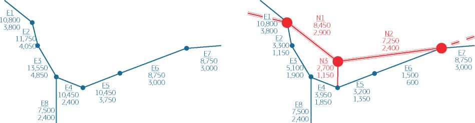
Year 20
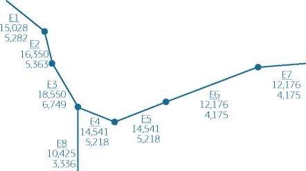
Legend: blue - existing sections, red - new sections. Section name, a.a.d.t. cars, a.a.d.t. LGV+HGV.
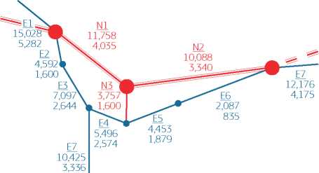
The level of service (LOS) is estimated according to the HCM methodology. Currently, LOS is D and E on some sections, which will deteriorate to F in near future. Once the motorway is constructed, the LOS on the existing road will improve to B and C, and will remain sufficient until year 20. The LOS on the motorway will reach C in year 20, which is an indication for adequate capacity.108
The cost estimate for works and supervision of the selected option is based on detailed design, as the works have not been tendered yet. Land purchase is partially completed. The cost estimate is based on constant prices of 2013.
|
Investment cost component |
Total cost |
|
Planning/design fees, technical assistance |
3,000,000 |
|
Land purchase |
12,000,000 |
|
Building and construction, of which: |
248,350,000 |
|
Earthworks |
12,500,000 |
|
Vegetation |
800,000 |
|
Road |
48,000,000 |
|
Bridges |
77,000,000 |
|
Tunnel |
80,000,000 |
|
retaining walls |
5,800,000 |
|
noise and safety barriers |
7,500,000 |
|
public utilities |
8,500,000 |
|
motorway information system |
1,250,000 |
|
Buildings |
1,000,000 |
|
other |
5,940,000 |
|
Plant and machinery |
0 |
|
Publicity |
60,000 |
|
Supervision |
5,000,000 |
|
Total Investment cost excl. contingencies |
268,350,000 |
|
Contingencies (10% of construction cost)109 |
24,835,000 |
|
Total Investment cost incl. contingencies |
293,185,000 |
|
VAT (recoverable) |
56,630,055 |
|
Total Investment cost including VAT |
349,815,055 |
The total project investment cost shown in the table above is considered eligible except the VAT, which is recoverable.
Estimates include all costs incurred for planning at feasibility stage and during the implementation period of the project, while the cost of all preliminary activities (pre-feasibility studies, surveys carried out before the feasibility study) are treated as a sunk cost and are thus not included.
Toll from freight vehicles is collected on behalf of the National Motorway Company by a toll collection company, through the pre-existing electronic toll collection system based on a combination of GPS and GSM technology. There is no physical investment necessary to extend the tolling on new sections, the motorway operator pays a fee for each toll transaction made on his road and receives the collected toll.
The following average unit costs were calculated to appraise the cost estimates of the most significant investment components, which were found to be well within the cost range of other comparable projects:
|
Investment component |
Unit cost |
|
Motorway, total |
EUR 16.3 million/km |
|
Motorway, excluding bridges and tunnels |
EUR 6.8 million/km |
|
Bridges |
EUR 1,151/m2 |
|
Tunnel |
EUR 18.2 million/km |
Routine maintenance cost for the new road is estimated on the basis of average maintenance requirements on the existing motorway network in the country and current maintenance practice of the motorway operator. Average routine maintenance cost is thus assumed to be EUR 34,000 per km of motorway110.
Routine maintenance cost for the existing road is assumed to be the same in the with and without-project scenarios and is thus excluded from the assessment.
Periodic maintenance of the new road is estimated on the basis of the expected schedule of periodic maintenance works. The timing of the works was determined on the basis of the observed maintenance cycle in the network of existing motorways in the country (e.g. re-pavement after 10 years, bridge repair after 15 years, retaining walls repair after 20 years, etc.); average cost of these works is also based on cost observed in the past.
Periodic maintenance of the existing road is excluded from the analysis. The decrease of traffic will extend the life of the infrastructure elements by a few years and consequently the maintenance cycle will be longer, however, it is assumed that maintenance measures will remain the same.
Operating cost of road includes toll collection cost; traffic management of the new section will be done from the existing traffic control centre without any additional cost and is thus excluded from the assessment. It is assumed that toll collection cost is EUR 0.12 per transaction (i.e. passage of a motorway section between the two junctions).
A toll is only collected from goods vehicles: for light goods vehicles (including buses) EUR 0.10 /km; for heavy goods vehicles EUR 0.20 /km. The assumed share of light goods vehicles (including buses) is 55 %, for heavy goods vehicles it is 45 %.
The analysis is performed using a 30-year reference period which is common for road projects. A residual value of the investment is considered at the end of the reference period; the residual value is EUR 13 million in the financial analysis which is calculated on the basis of the net present value of cash flows generated after the reference period (based on the perpetuity formula) and EUR 150 million in the economic analysis (based on the depreciation formula and corrected by the conversion factor). The financial and economic analyses use constant prices. A real discount rate of 4 % is used in the financial calculations, while a 5.0 % social discount rate is used in the economic analysis, in line with EU wide benchmark set by the Commission. VAT is reimbursable and thus excluded from the analysis.
The cash-flows for the financial analysis are shown in the following table, including the calculation of the relevant financial performance indicators of the project.
The markedly negative financial net present value of the investment (FNPV(C) = -EUR 248 million) shows that the project requires EU assistance to make it viable.
The project is a net revenue generating operation in the meaning of Article 61 of Regulation (EU) 1303/2013. In this case, the contribution from the EU Cohesion Fund to the project has been determined using the method based on the calculation of the discounted net revenue111. The resulting pro-rata application of discounted net revenue is 93.4 %. This, multiplied with the eligible cost shown in section IV above (EUR 293.2 million) and with the co-financing rate of the relevant priority axis of the OP (85 %), gives a EU grant for the project of EUR 232.7 million.
The remainder of the investment is provided by the promoter entirely from equity, without the need to contract loans. The equity contribution will be financed through additional paid-in capital from the State, for which a formal commitment exists.
|
EU GRANT |
1 |
2 |
3 |
4 |
5 |
6 |
7 |
8 |
9 |
10 |
15 |
20 |
25 |
30 | ||
|
Construction |
Operation | |||||||||||||||
|
Calculation of Discounted Investment Cost (DIC) |
NPV 4 % | |||||||||||||||
|
Investment cost (excluding contingencies) |
mEUR |
259.7 |
103.6 |
101.8 |
63.0 |
0.0 |
0.0 |
0.0 |
0.0 |
0.0 |
0.0 |
0.0 |
0.0 |
0.0 |
0.0 |
0.0 |
|
DIC / Investment cost cash-flow |
mEUR |
259.7 |
103.6 |
101.8 |
63.0 |
0.0 |
0.0 |
0.0 |
O d |
O b |
O d |
0.0 |
0.0 |
0.0 |
0.0 |
0.0 |
|
Calculation of Discounted Net Revenues (DNR) |
NPV 4 % | |||||||||||||||
|
Revenue |
mEUR |
40.9 |
0.0 |
0.0 |
0.0 |
2.2 |
2.3 |
2.3 |
2.4 |
2.4 |
2.5 |
2.5 |
2.7 |
2.9 |
3.1 |
3.4 |
|
O&M costs |
mEUR |
27.9 |
0.0 |
0.0 |
0.0 |
0.9 |
0.9 |
0.9 |
0.9 |
0.9 |
0.9 |
0.9 |
7.8 |
0.9 |
1.0 |
1.0 |
|
Residual value of investments |
mEUR |
4.2 |
0 |
0 |
0 |
0 |
0 |
0 |
0 |
0 |
0 |
0 |
0 |
0 |
0 |
13 |
|
DNR / Net revenue cash-flow |
mEUR |
17.2 |
0.0 |
0.0 |
0.0 |
1.4 |
1.4 |
1.5 |
1.5 |
1.5 |
1.6 |
1.6 |
-5.1 |
2.0 |
2.2 |
15.6 |
|
ELIGIBLE COST (EC) |
mEUR |
293.2 |
|
Pro-rata application of DNR = (DIC - DNR) / DIC |
93.4% | |
|
CO-FINANCING RATE OF PRIORITY AXIS (CF) |
85.0% |
EU GRANT ( = EC x PRO-RATA x CF)
mEUR
232.7
|
FRR(C) |
1 |
2 |
3 |
4 |
5 |
6 |
7 |
8 |
9 |
10 |
15| |
20 |
25 |
30 | ||
|
Construction |
Operation | |||||||||||||||
|
Calculation of the Return on Investment |
NPV 4 % | |||||||||||||||
|
Investment cost (excluding contingencies) |
mEUR |
-259.7 |
-103.6 |
-101.8 |
-63.0 |
0.0 |
0.0 |
0.0 |
0.0 |
0.0 |
0.0 |
0.0 |
0.0 |
0.0 |
0.0 |
0.0 |
|
O&M cost |
mEUR |
-27.9 |
0.0 |
0.0 |
0.0 |
-0.9 |
-0.9 |
-0.9 |
-0.9 |
-0.9 |
-0.9 |
-0.9 |
-7.8 |
-0.9 |
-1.0 |
-1.0 |
|
Revenue |
mEUR |
40.9 |
0.0 |
0.0 |
0.0 |
2.2 |
2.3 |
2.3 |
2.4 |
2.4 |
2.5 |
2.5 |
2.7 |
2.9 |
3.1 |
3.4 |
|
Residual value of investments |
mEUR |
4.2 |
0.0 |
0.0 |
0.0 |
0.0 |
0.0 |
0.0 |
0.0 |
0.0 |
0.0 |
0.0 |
0.0 |
0.0 |
0.0 |
13.2 |
|
FNPV(C) - before EU grant / Net cash-flow |
mEUR |
-248.2 |
-103.6 |
-101.8 |
-63.0 |
1.4 |
1.4 |
1.5 |
1.5 |
1.5 |
1.6 |
1.6 |
-5.1 |
2.0 |
2.2 |
15.6 |
FRR(C) - before EU grant -8.8%
|
FRR(K) |
12 3 |
4 5 6 7 8 9 10 15 20 25 30 | |
|
Construction |
Operation | ||
|
National Financing Sources | |||
|
Promoter's contribution |
mEUR |
24.0 22.5 13.9 0.0 0.0 0.0 0.0 0.0 0.0 0.0 0.0 0.0 0.0 0.0 | |
|
Calculation of the Return on National Capital |
NPV 4 % | |||||||||||||||
|
Promoter's contribution |
mEUR |
-58.6 |
-24.0 |
-22.5 |
-13.9 |
0.0 |
0.0 |
0.0 |
0.0 |
0.0 |
0.0 |
0.0 |
0.0 |
0.0 |
0.0 |
0.0 |
|
O&M cost |
mEUR |
-27.9 |
0.0 |
0.0 |
0.0 |
-0.9 |
-0.9 |
-0.9 |
-0.9 |
-0.9 |
-0.9 |
-0.9 |
-7.8 |
-0.9 |
-1.0 |
-1.0 |
|
Revenue |
mEUR |
40.9 |
0.0 |
0.0 |
0.0 |
2.2 |
2.3 |
2.3 |
2.4 |
2.4 |
2.5 |
2.5 |
2.7 |
2.9 |
3.1 |
3.4 |
|
Residual value of investments |
mEUR |
4.2 |
0.0 |
0.0 |
0.0 |
0.0 |
0.0 |
0.0 |
0.0 |
0.0 |
0.0 |
0.0 |
0.0 |
0.0 |
0.0 |
13.2 |
|
FNPV(K) - after EU grant / Net cash-flow |
mEUR |
-41.4 |
-24.0 |
-22.5 |
-13.9 |
1.4 |
1.4 |
1.5 |
1.5 |
1.5 |
1.6 |
1.6 |
-5.1 |
2.0 |
2.2 |
15.6 |
FRR(K) - after EU grant -2.9%
Note that the FNPV(K) on national capital remains negative because the EU grant is covering only 85 % of the gap, while the remainder is covered by a national public grant.
The project appears to be financially sustainable, as the investment cost during implementation is covered by an equal amount in financing sources and its cumulated net cash flow during operations is positive during the entire evaluation period.
FINANCIAL SUSTAINABILITY
|
12 3 |
4 5 6 7 8 9 10 15 20 25 30 |
|
Construction |
Operation |
Verification of the Financial Sustainability of the Project
|
EU grant |
mEUR |
|
Promoter's contribution |
mEUR |
|
Revenue |
mEUR |
|
Total cash inflows |
mEUR |
|
Investment cost (including contingencies) |
mEUR |
|
O&M cost |
mEUR |
|
Total cash outflows |
mEUR |
|
Net cash-flow |
mEUR |
|
Cumulated net cash-flow |
mEUR |
|
88.4 |
89.2 |
55.1 |
0.0 |
0.0 |
0.0 |
0.0 |
0.0 |
0.0 |
0.0 |
0.0 |
0.0 |
0.0 |
0.0 |
|
24.0 |
22.5 |
13.9 |
0.0 |
0.0 |
0.0 |
0.0 |
0.0 |
0.0 |
0.0 |
0.0 |
0.0 |
0.0 |
0.0 |
|
0.0 |
0.0 |
0.0 |
2.2 |
2.3 |
2.3 |
2.4 |
2.4 |
2.5 |
2.5 |
2.7 |
2.9 |
3.1 |
3.4 |
|
112.4 |
111.7 |
69.0 |
2.2 |
2.3 |
2.3 |
2.4 |
2.4 |
2.5 |
2.5 |
2.7 |
2.9 |
3.1 |
3.4 |
|
-112.4 |
-111.7 |
-69.1 |
0.0 |
0.0 |
0.0 |
0.0 |
0.0 |
0.0 |
0.0 |
0.0 |
0.0 |
0.0 |
0.0 |
|
0.0 |
0.0 |
0.0 |
-0.9 |
-0.9 |
-0.9 |
-0.9 |
-0.9 |
-0.9 |
-0.9 |
-7.8 |
-0.9 |
-1.0 |
-1.0 |
|
-112.4 |
-111.7 |
-69.1 |
-0.9 |
-0.9 |
-0.9 |
-0.9 |
-0.9 |
-0.9 |
-0.9 |
-7.8 |
-0.9 |
-1.0 |
-1.0 |
|
0.0 |
0.0 |
0.0 |
1.4 |
1.4 |
1.5 |
1.5 |
1.5 |
1.6 |
1.6 |
-5.1 |
2.0 |
2.2 |
2.4 |
|
0.0 |
0.0 |
0.0 |
1.4 |
2.8 |
4.3 |
5.8 |
7.3 |
8.9 |
10.5 |
12.3 |
14.3 |
15.6 |
20.3 |
Economic analysis
For the purpose of socio-economic assessment, the investment cost estimate was corrected for fiscal effects by factor 0.91 (excl. cost of land which was not subject to fiscal correction). The routine maintenance cost was corrected by factor 0.88. Fiscal correction factors are based on share of transfer payments in labour and energy cost and their respective share in overall cost.
The socio-economic analysis includes following monetised benefits, which are consistent with the project objectives, i.e. faster travel on a safer road with separated carriageways, travel time savings, vehicle operating cost savings, accident cost savings.
Project benefits, related to the reduction of negative impacts (pollution and noise) within settlements were not quantified, given that these were not considered to be of importance in monetary terms, but the socio-economic analysis does include project impact on the emission of CO2 as the main global environmental impact of transport.
Travel time savings (in minutes saved per person) are quantified with the help of the traffic model on the basis of average speeds achieved by cars and goods vehicles on the existing and new road links (see table below), their length and assumed traffic volumes. As a consequence of the project, it is estimated that the average car using the full length of the new motorway will save around 12 minutes in year 1, while goods vehicles will save around nine minutes. Time savings for vehicles remaining on existing road are around four minutes per vehicle.
Average speed (km/h)
|
Section |
Length (km) |
Without project |
With project | ||||||
|
Year 1 |
Year 20 |
Year 1 |
Year 20 | ||||||
|
Cars |
LGV+ HGV |
Cars |
LGV+ HGV |
Cars |
LGV+ HGV |
Cars |
LGV+ HGV | ||
|
E2 |
1.7 |
51.4 |
46.5 |
41.0 |
40.2 |
64.7 |
53.8 |
62.5 |
53.4 |
|
E3 |
3.6 |
35.2 |
35.2 |
31.9 |
31.9 |
38.8 |
38.6 |
32.5 |
32.4 |
|
E4 |
3.1 |
42.7 |
42.1 |
32.3 |
31.8 |
57.2 |
53.0 |
52.9 |
49.6 |
|
E5 |
3.7 |
40.6 |
39.3 |
34.5 |
33.9 |
54.8 |
51.0 |
53.9 |
50.2 |
|
E6 |
5.6 |
69.0 |
57.6 |
55.1 |
47.5 |
79.1 |
63.6 |
78.7 |
63.6 |
|
N1 |
5.7 |
104.8 |
75.2 |
98.4 |
72.4 | ||||
|
N2 |
10.7 |
113.0 |
74.5 |
107.7 |
72.5 | ||||
|
N3 |
2.0 |
79.7 |
70.0 |
78.6 |
69.6 | ||||
To monetise the benefit of VOT savings, the following additional assumptions114 were made:
|
Variable |
Assumption |
Comment |
|
Average occupancy, cars |
1.8 persons |
Based on different surveys carried out in the country |
|
Average occupancy, goods vehicles |
1.2 persons | |
|
Trip purpose mix, cars |
20 % work trips 80 % non-work trips | |
|
Trip purpose mix, goods vehicles |
100 % work trips | |
|
Unit value of time, work trips |
EUR 12.90 per hour |
Estimate based on average wage in the country (EUR 9 per hour) and assumed labour related overhead (33 %) |
|
Unit value of time, non-work trips |
EUR 4.30 per hour |
Estimated at 1/3 of value of time for work trips |
|
Escalation factor for VOT |
GDP per capita growth, with elasticity factor of 0.7 |
Vehicle operating costs (VOC) savings are calculated for different types of vehicles taking into consideration national vehicle fleet, speed and road capacity, road condition and road geometry. The software used applies nationally calibrated values and crew cost has been excluded to avoid double-counting.
Accident cost savings are related to the fact that the majority of the traffic will be diverted to a safer motorway, with separated carriageways for each direction and grade-separated crossings with lower category roads. Analyses of traffic safety revealed that the traffic fatality risk on the existing road is 10.7 fatalities per one billion vehicle-km, whereas on a motorway it is 3.1 fatalities per one billion vehicle-km. It was estimated that the construction of the new road will save around 0.6 fatalities in the opening year and around 0.9 fatalities in the final year of analysis.
A prevented road fatality in the country is estimated at EUR 677,500 (estimate based on values derived from a literature review). It is assumed that this value will grow at the same rate as real GDP per capita, with an elasticity factor of 1.0.
CO2 savings are related to the fact that due to the more favourable alignment the distance travelled for the majority of the traffic will reduce, while the traffic flow remaining on the existing road will be smoother. The assumed unit cost is EUR 31 per tonne of CO2 (in 2013 prices), with an annual growth of EUR 1.
The resulting cash flows and their ENPVs are shown in the following table. 112
|
ERR |
12 3 |
4 5 6 7 8 9 10 15 20 25 30 | ||||||||||||||
|
Construction |
Operation | |||||||||||||||
|
Calculation of the Economic Rate of Return |
NPV 5.0 % | |||||||||||||||
|
Project investment cost |
mEUR |
-234.3 |
-94.9 |
-92.1 |
-57.0 |
0.0 |
0.0 |
0.0 |
0.0 |
0.0 |
0.0 |
0.0 |
0.0 |
0.0 |
0.0 |
0.0 |
|
Project O&M costs |
mEUR |
-21.0 |
0.0 |
0.0 |
0.0 |
-0.8 |
-0.8 |
-0.8 |
-0.8 |
-0.8 |
-0.8 |
-0.8 |
-6.9 |
-0.8 |
-0.8 |
-0.9 |
|
Residual value of investments |
mEUR |
44.6 |
0.0 |
0.0 |
0.0 |
0.0 |
0.0 |
0.0 |
0.0 |
0.0 |
0.0 |
0.0 |
0.0 |
0.0 |
0.0 |
151.0 |
|
Total economic costs |
mEUR |
-210.7 |
-94.9 |
-92.1 |
-57.0 |
-0.8 |
-0.8 |
-0.8 |
-0.8 |
-0.8 |
-0.8 |
-0.8 |
-6.9 |
-0.8 |
-0.8 |
150.2 |
|
B1. Time savings |
mEUR |
266.7 |
0.0 |
0.0 |
0.0 |
10.7 |
11.5 |
12.3 |
13.2 |
14.1 |
15.0 |
16.0 |
20.7 |
25.4 |
30.5 |
37.7 |
|
B2. VOC savings |
mEUR |
26.5 |
0.0 |
0.0 |
0.0 |
1.3 |
1.4 |
1.5 |
1.5 |
1.6 |
1.7 |
1.8 |
2.1 |
2.4 |
2.7 |
3.0 |
|
B3. Accident savings |
mEUR |
9.2 |
0.0 |
0.0 |
0.0 |
0.4 |
0.4 |
0.5 |
0.5 |
0.5 |
0.5 |
0.6 |
0.7 |
0.9 |
1.0 |
1.2 |
|
B4. CO2 savings |
mEUR |
3.1 |
0.0 |
0.0 |
0.0 |
0.1 |
0.1 |
0.1 |
0.1 |
0.1 |
0.2 |
0.2 |
0.2 |
0.3 |
0.4 |
0.5 |
|
Total economic benefits (B1+B2+B3+B4) |
mEUR |
305.5 |
0.0 |
0.0 |
0.0 |
12.5 |
13.5 |
14.4 |
15.4 |
16.3 |
17.4 |
18.5 |
23.7 |
28.9 |
34.6 |
42.3 |
|
ENPV / Net benefits |
mEUR |
87.0 |
-94.9 |
-92.1 |
-57.0 |
11.8 |
12.8 |
13.7 |
14.6 |
15.5 |
16.6 |
17.7 |
16.8 |
28.1 |
33.7 |
192.5 |
ERR 7.1 %
B/C RATIO 1.45
In terms of ENPV, the main benefit of the project are travel time savings (87 % of total), followed only distantly by vehicle operating cost savings (9 %), accident cost savings (3 %), and CO2 savings (1 %). All in all, the results of the socio-economic analysis (ERR: 7.1 %, ENPV: EUR 87.0 million) show that the project generates a positive welfare change and is thus worthy of receiving EU assistance.
This is performed by calculating the percentage change of the FNPV(C) and the ENPV as a consequence of a 1 % change in key costs and benefits. If the absolute percentage change in ENPV is higher than 1 %, then the respective variable is deemed to be critical.
|
Variable tested |
FNPV(C) elasticity |
ENPV elasticity |
|
Investment cost +1 % |
-1.07 % |
-2.70 % |
|
Traffic on new road +1 % |
+ 0.27 % |
+ 2.04 % |
|
O&M cost +1 % |
-0.12 % |
-0.24 % |
|
Toll revenue +1 % |
+ 0.17 % |
n.a. |
|
VOT +1 % |
n.a. |
+ 3.08 % |
|
VOC +1 % |
n.a. |
+ 0.31 % |
|
Accident saving +1 % |
n.a. |
+ 0.11 % |
|
CO2 saving +1 % |
n.a. |
+ 0.03 % |
The sensitivity analysis reveals that the project's financial performance is not very sensitive to any change in the input variables.
On the other hand, the economic performance is quite sensitive to changes in assumed investment cost and demand and value of travel time savings, which are considered critical variables. This is also reflected in their switching values (i.e. necessary changes in the variables for the ENPV to become negative), which are +37 % for the investment cost and -32 % for the VOT savings (as compared to the base case assumptions). Given that these values are, broadly speaking, within realistic possibilities, it was decided to carry out a probabilistic risk analysis in addition to the standard qualitative risk analysis.
Given that the sensitivity analysis revealed no critical variables for the financial analysis, the risk analysis concentrates - for the sake of simplicity - solely on the economic analysis of the project and is done in both qualitative and quantitative terms.
The qualitative risk analysis is presented in the following risk matrix. It takes into account uncertainties related to all aspects of the project. Note that prevention and mitigation measures are only defined for the remaining risks of the highest level.
|
Risk |
Effect |
Probability (P) |
Severity (S) |
Risk level |
Causes |
Prevention/mitigation measures |
|
PLANNING AND ADMINISTRATIVE RISKS | ||||||
|
Building permit acquisition |
delay |
A |
III |
Low |
EIA completed, documentation for building permit is ready. | |
|
Utilities (and other) approvals |
delay |
A |
I |
Low |
Approvals obtained, coordination on-going, spatial plan is prepared and approved. | |
|
Changes in environmental requirements |
A |
I |
Low |
EIA procedure carried out. | ||
|
LAND ACQUISITION | ||||||
|
Cost of land |
cost |
B |
III |
Low |
Land purchase partially completed. | |
|
Delays of land purchasing |
delay |
B |
IV |
moderate |
Land purchase partially completed. | |
|
Additional requirements |
cost |
A |
I |
Low |
No additional requirements appeared so far. | |
|
Land for temporary access to the site |
A |
I |
Low |
Construction site accessible, no need for temporary access. | ||
|
DESIGN | ||||||
|
Inadequate site surveys and investigation |
cost |
A |
III |
Low |
Surveys were undertaken during design, conditions known. | |
|
Changes in the requirements |
cost |
A |
III |
low |
All infrastructure components/ parameters agreed. | |
|
Inadequate design cost estimates |
cost |
B |
III |
low |
Design mainly completed. | |
|
CONSTRUCTION RISKS | ||||||
|
Inadequate construction cost estimates (compared to received bids) |
cost |
D |
IV |
high |
Tender price not yet known. |
Decision to submit the application for EU funds depending on tender results, contingencies included in the budget, credit line for additional funding is available |
|
Cost overruns (during construction) |
cost |
D |
IV |
high |
Project implementation did not start yet, it includes a tunnel construction which involves geological risks. |
Surveys were undertaken during design, design was audited |
|
Inadequate construction quality |
cost |
C |
III |
moderate |
Estimate based on experience. | |
|
Flooding, landslides and similar |
cost |
A |
III |
low | ||
|
Archaeological findings |
cost |
B |
I |
low |
No known archaeological findings in adjacent areas. | |
|
Inadequate supervision cost estimates |
cost |
C |
I |
low |
Tender price not yet known. | |
|
Inadequate temporary works cost estimates |
cost |
C |
I |
low |
Project implementation did not start yet, cost compared to total cost is low. | |
|
Contractor’s bankruptcy |
delay |
B |
III |
low |
Possible, adequate requirements concerning financial strength will be included in tender dossier. | |
|
Risk |
Effect |
Probability (P) |
Severity (S) |
Risk level |
Causes |
Prevention/mitigation measures |
|
Contractor’s resources |
delay |
B |
III |
low |
Financial situation may affect contractor’s ability to finance works and the stock of materials. | |
|
Public procurement |
delay |
C |
III |
moderate |
Could be delayed by a year (experience). | |
|
OTHER RISKS | ||||||
|
Protester action |
cost |
A |
I |
low |
Master plan approved, no civil initiatives active. | |
|
Change of strategy |
cost |
A |
I |
low |
High priority project for the country, international commitments, low cost invested so far. | |
|
Introduction of direct tolls (toll evasion) |
% traffic |
B |
III |
low |
Vignette system, no intention to introduce direct tolling of the cars at the moment, transiting trucks will be prohibited to use lower category roads. | |
|
Lack of national finance |
delay |
A |
IV |
moderate |
Reduced capacity to fund projects, but project remains high priority. | |
|
Traffic (demand) risk |
% traffic |
C |
IV |
high |
Traffic study available, uncertainties regarding long term forecast. |
Audit the traffic model. |
Evaluation scale: Probability: A. Very Unlikely; B. Unlikely; C. About as likely as not; D. Likely; E. Very likely.
Severity: I. No effect; II. Minor; III. Moderate; IV. Critical; V. Catastrophic.
Risk level: Low; Moderate; High; Unacceptable.
The qualitative risk analysis basically displays two critical risks: i) construction cost risk (increase of contract price compared to designer's estimate; increase of out-turn cost compared to contract price, amongst others due to considerable geological risk); and ii) demand risk.
These two risks were therefore subject to a quantitative risk analysis.
A Monte Carlo risk simulation was used to assess the probability distribution of the project's socio-economic performance indicators (ENPV), repeated in 4,000 iterations. An asymmetrical triangular probability distribution was applied113, with the following assumptions concerning possible ranges for investment cost and traffic benefits (min., max.):
• investment cost (-5 %; +20 %);
• traffic on the new road (-30 %; +15 %).
The assumed range of investment cost is based on ex-post evaluation of motorway projects in the past which analysed cost development during the project cycle, and which found that for standard project final out-turn cost is in the range of -5 % to +20 % compared to the designer's estimate.
Monte Carlo analysis simulates the variation of the traffic on the new road which affects the related benefits (time savings, vehicle operating cost, accident savings). The parameters (min., max.) were derived through panel assessment which considered sporadic evidence for some of the projects and published articles. Probability density and cumulative probability distributions for the ENPV are shown below. In the base scenario the ENPV is around EUR 87 million, the most likely risk adjusted ENPV is around EUR 77 million. The probability of negative ENPV is 15 %.
Probability density of ENPV
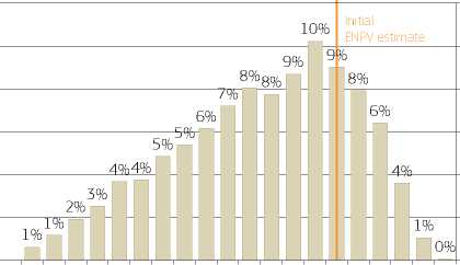
12%
10%
8%
6%
4%
2%
0%
<-°> , Jo Jo Jb JV o°> q\ JV Jo Jo Jb Jb \ o. <p Jo Jb
p- P' p p' } y P' p Py P P' <o>' P P P'jP'jP'jP'
0%
Cumulative probability distribution
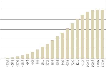
12%
10%
8%
6%
4%
2%
0%
The risk analysis suggests that there is a probability for a negative ENPV due to residual risks that are outside of the project promoter’s control, namely geological conditions where a tunnel is to be built (geological survey cannot exclude all risks), construction market prices (tender prices not always following the experience of previous projects) and demand (traffic behaviour not always following foreseeable patterns). All necessary risk prevention measures have already been undertaken during project design, such as detailed geological and hydrological surveys, and the elaboration of a traffic model which provided parameters for dimensioning of the road elements. As a mitigation measure regarding traffic forecast, a recommendation is to audit the traffic model and continuously improve it, if and where necessary, e.g. by obtaining the latest input data to feed into the model.
Considering the careful project preparation process thus far (incl. risk prevention measures) and the positive expected ENPV, the calculated risk of negative ENPV is deemed acceptable and the project should be released for the next stage (tendering). Nevertheless, the final approval of the project and application for EU funding are not forthcoming until the results of tender are known. If the tender would result in significantly higher prices than estimated (i.e. more than 10 %) it is recommended repeating the CBA and risk analysis with new inputs and reconsidering the further project development and implementation.
The project consists of the upgrading of a double-track railway section, part of the TEN-T Priority axis Y. The existing line is 94.75 km long (from the Y end of station A to the X end of station B), all double tracked, electrified and equipped with automatic line block, and is used for both passenger and freight traffic114.
Current traffic averages approximately 40 pairs of trains per day. The average technical speed allowed by the current condition of the line is about 81 km/h (design speed equivalent, commercial speed is lower). The line is not interoperable as it is not equipped with ERTMS (European Rail Traffic Management System). The main performance problems of the existing line are caused by the speed limiting alignment parameters and by the significant lack of past maintenance.
Further to the realignments (speed upgrade variants) provided under the project, the section length shall be reduced from 94.75 km to 89.5 km. The project works include notably:
• renewal of 63.464 double track km on the existing alignment and construction of 26.036 double track km on a new alignment. Upon upgrading, approximately 60 % of the line section will allow a maximum speed of 160 km/h;
• construction of two single pipe tunnels of 1,260 m total length;
• construction of 13.705 km retaining walls and 1.260 km slope protection and river bed correction.
• renewal or repair of 32 bridges, construction or repair of 106 culverts;
• rehabilitation of passenger buildings in four stations and six halts (about 14,725 m2);
• enlargement and protection of station platforms, construction of 6 pedestrian tunnels and repair of a grade crossings;
• reduction or re-arrangement of station tracks, replacement of 144 turnouts, extension of freight siding to 750 m length;
• installation of 7 Electronic Interlockings, ERTMS Level 2 including GSM-R and rehabilitation of the existing Automatic Train Protection (INDUSI/PZB type) system as fall-back;
• closure of 7 existing level crossings, replacement of two level crossing by overpasses and installation of automatic protection systems with four half barriers for the remaining 33 level crossings;
• rehabilitation/installation of the electric traction system on the entire length of 89.5 km;
• rehabilitation of telecommunication systems (voice and data communication, passenger information equipment, two transmission lines based on optic fibre).
The following design parameters were applied in consideration of the applicable standards/targets:
|
Criteria |
Parameter |
|
Maximum speed of passenger trains |
160 km/h (on approx. 60 % of line length), 120 km/h on the rest |
|
Maximum speed of freight trains |
120 km/h |
|
Clearance |
UIC - B. |
|
Maximum axle load |
22.5 t |
|
Maximum gradient |
12.5 %o (within this section the max. gradient will be only 3%o). |
|
Minimum length of sidings |
750 m |
|
Distance between axis in open line |
4.20 m |
|
Distance between axis in stations |
At least 4.75 m (Article 29(3) RET), but regularly 5.00 m. |
|
Height of platforms in stations |
55 cm |
|
Level crossings |
Automatic 4 half barriers + CCTV |
|
Compatibility of signal equipment |
ERTMS Level 2 with LS/Indusi ATP as fall-back |
Fundamentally the project aims to improve the level of railway service on an important corridor, in particular by reducing travel times, increasing capacity and improving safety, thereby contributing to the overall attractiveness of the rail transport mode within the country and also at trans-European level.
Specifically, the upgrade towards the target speed of 160 km/h for passenger and 120 km/h for freight trains (within ERTMS Level 2 environment) will allow a travel time reduction from the current approximately 96 to 55 minutes journey time for long distance passenger trains.
The main results expected are:
• reducing the travel time for the existing rail users;
• reducing operating costs for service providers;
• diverting traffic from road to rail with benefits for travellers as well as for society through a reduction of external costs and attracting new traffic to rail; and
• improving traffic safety.
The project is consistent with both the existing strategic national and EU (TEN-T) plans and the priorities of the Operational Programme Transport (OPT). It contributes to the achievement of the following OPT indicators:
|
Indicator |
Unit |
Target 2015 |
|
Output | ||
|
Total length of reconstructed or upgraded railway lines |
km |
209.18 |
|
Result | ||
|
Value of time savings for passengers and freight transported by upgraded railways |
M EUR/year |
86.93 |
The following main alternatives have been studied within the feasibility study:
Assumes the business as usual scenario, under which the railway infrastructure company continues to operate the line following current trends, i.e. with the current level of both routine and periodic maintenance (slightly lower than required) -with the effect of continuing the slight trend of lowering the average speed (by approx. 0.5 % per year) of the line in time.
• Alternative 1: Online rehabilitation of the line to the initial design speed (120 km/h) without any new upgrades/new alignments.
• Alternative 2: Moderate speed upgrade to 160 km/h on approx. 60 % of the line by 2020 - where this could be achieved with low to moderate investment costs (avoiding very costly structures such as long tunnels and bridges).
• Alternative 3: Maximal speed upgrade to 160 km/h on approx. 80 % of the line by 2020.
The alternatives have been compared within the feasibility study on the basis of CBA, as well as other considerations (such as environmental impact including on Natura 2000 areas) and Alternative 2, providing the best economic return (highest ERR and B/C ratio), was selected as the preferred option115 - which was taken forward to detailed design and is the subject of this analysis.
The current traffic volumes (average between A and B) are approximately:
• 30 pairs of passengers trains/day (approx. 4,900 pax/day);
• 9 pairs of freight trains/day (approx. 12,000 ton/day).
The forecast is derived from a model based on the impact of exogenous (GDP growth, population growth, motorisation, travel time by road, fuel cost growth) and endogenous (travel time by rail, rail fare growth) factors - with appropriate calibration.
During implementation the impact of the project is negative,reflecting the disruptions over the construction period, then gradually positive after adding operation of the corridor. The positive effect reflects additional traffic mainly diverting from roads - as a result of travel time savings.
Overall, the forecast results in an average incremental growth of the railway traffic, roughly equivalent to 1.1 % per annum. for passengers and 0.4 % per annum for freight over the appraisal period. The traffic forecast results without and with - project are illustrated in the graphics below:
Passengers traffic
-without project
-with project
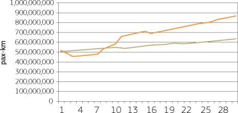
-without project
-with project
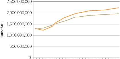
1 4 7 10 13 16 19 22 25 28
Freight traffic
The cost estimate for works and supervision of the selected option is based on a detailed design estimate (broken down transparently into quantities and unit costs per components). The works have not been tendered yet and land purchase is partially completed. The cost estimate is made at constant prices of year Y.
|
In EUR |
Total Project costs |
Ineligible costs |
Eligible costs | |
|
(A) |
(B) |
(C)=(AHB) | ||
|
1 |
Planning/design fees |
14,024,673, |
, |
14,024,673, |
|
2 |
Land purchase |
12,756,615 |
, |
12,756,615 |
|
3 |
Building and construction |
648,131,978 |
, |
648,131,978 |
|
4 |
Plant and machinery |
38,354,080 |
, |
38,354,080 |
|
5 |
Contingencies |
51,721,770 |
, |
51,721,770 |
|
6 |
Price adjustment (if applicable) |
0 |
, |
0 |
|
7 |
Technical assistance |
0 |
, |
0 |
|
8 |
Publicity |
125,747 |
, |
125,747 |
|
9.1 |
Supervision |
13,111,376 |
3,255,491117 |
12,855,885 |
|
9.2 |
Other costs |
922,259 |
922,259 | |
|
10 |
Sub-TOTAL |
779,148,498 |
255,491 |
778,893,007 |
|
11 |
VAT |
186,995,640 |
186,995,640 |
0 |
|
12 |
TOTAL |
966,144,137 |
187,251,131 |
778,893,007 |
The average cost per (double-track) km of the project, including ancillary investments in stations, etc. is approx. EUR 8.7 million (ex-VAT), which is in line with similar projects in the country.
The average maintenance unit costs for the railway line used in the analysis are:
• for the ‘without project' scenario - EUR 29,717 per track km per year (as per actual costs incurred over the last 5 years -reflecting the business as usual assumptions);
• for the ‘with project' scenario - EUR 37,500 per track km per year, as estimated for good maintenance standards based on local costs
Another factor influencing the overall O&M expenditure of the project is the reduction in the length of the rail section. Overall, however, there would be an increase in the O&M costs in the ‘with' project scenario as compared to the ‘without' project scenario.
The diversion of traffic from roads may have a marginal impact (reduction) on the road O&M, but this is usually considered not significant enough for appraisal and is therefore ignored.
The residual value has been calculated as the net present value of the financial/economic flows118 over the remaining lifetime (52 years) outside the reference period (30 years). This method is considered to reflect more realistically the actual value of the assets than the traditional ‘accounting' method based on linear depreciation.
The analysis is performed using a 30-year reference period which is common for railway projects.
The financial and economic analyses use constant prices (year Y). A 4 % discount rate in real terms is used in the financial calculations, while a 5 % social discount rate is used in the economic analysis, in line with EU wide benchmark set by the Commission. VAT is excluded from the analysis since it is recoverable.
Since the line is operated by more than one operator the financial analysis is done from the perspective of the infrastructure owner/manager; therefore the relevant revenues are the track access charges (TAC) paid by the freight and passengers operators.
Additional revenues are generated by the project as a result of the incremental traffic (trains-km) forecasted within the traffic analysis. The calculation is based on the current level of the track access charges (i.e. average EUR 2.11 /train-km for passengers and EUR 3.29 /train-km for freight), which is assumed not to change in real terms over the appraisal period. The choice of not raising the level of the TAC following the line upgrading was made on the basis of the policy line taken in terms of transferring maximum benefits of the upgrade to the end users (rather than trying to recover part of it) - in view of improving the attractiveness of the rail mode and thus contributing to the mode shift objective. Note also a temporary drop in revenues during the three years of the construction period as a result of the disruptions inherent to the works under operation (track capacity limitations, delays, etc.).
The project is a net revenue generating operation in the meaning of Article 61 of Regulation (EU) 1303/2013. To determine the contribution of the Cohesion Fund to the project, the method based on the calculation of the discounted net revenue was applied119, which is shown in the following table. The analysis shows that the project is not able to repay around 95 % of the invested capital.
|
12 3 |
4 5 6 7 8 9 10 15 20 25 30 |
|
Construction |
Operation |
EU GRANT
|
Calculation of the Discounted Investment Cost (DIC) |
NPV 4% | |||||||||||||||
|
Investment cost (excluding contingencies) |
mEUR |
670.8 |
227.2 |
214.4 |
285.9 |
0.0 |
0.0 |
0.0 |
0.0 |
0.0 |
0.0 |
0.0 |
0.0 |
0.0 |
0.0 |
0.0 |
|
DIC / Investment cost cash-flow |
mEUR |
670.8 |
227.2 |
214.4 |
285.9 |
0.0 |
0.0 |
0.0 |
0.0 |
0.0 |
0.0 |
0.0 |
0.0 |
0.0 |
0.0 |
0.0 |
|
Calculation of the Discounted Net Revenues (DNR) |
NPV 4% | |||||||||||||||
|
Revenue (track access charges) |
mEUR |
35.1 |
-0.1 |
-0.1 |
-0.2 |
0.2 |
0.4 |
0.8 |
1.2 |
1.5 |
2.3 |
2.4 |
2.8 |
3.2 |
3.7 |
4.1 |
|
O&M cost |
mEUR |
-15.7 |
0.0 |
0.0 |
0.0 |
-1.1 |
-1.1 |
-1.1 |
-1.1 |
-1.1 |
-1.1 |
-1.1 |
-1.1 |
-1.1 |
-1.1 |
-1.1 |
|
Residual value of investments |
mEUR |
13.7 |
0.0 |
0.0 |
0.0 |
0.0 |
0.0 |
0.0 |
0.0 |
0.0 |
0.0 |
0.0 |
0.0 |
0.0 |
0.0 |
44.3 |
|
DNR / Net revenue cash-flow |
mEUR |
33.1 |
-0.1 |
-0.1 |
-0.2 |
-0.9 |
-0.7 |
-0.3 |
0.1 |
0.5 |
1.2 |
1.3 |
1.7 |
2.2 |
2.6 |
47.4 |
|
ELIGIBLE COST (EC) |
mEUR |
778.9 |
|
Pro-rata application of DNR = (DIC - DNR) / DIC |
95.1% | |
|
CO-FINANCING RATE OF THE PRIORITY AXIS (CF) |
85.0% |
EU GRANT ( = EC x PRO-RATA x CF) mEUR 629.4
In this case, the EU grant has been calculated by multiplying the eligible cost shown in section IV above (EUR 778.9 million) by the pro-rata application of discounted net revenue (95.1 %) and the co-financing rate of the relevant priority axis of the OP (85 %) - resulting in EUR 629.4 million. The remainder of the investment is co-financed out of national (state-budget and railway company120) funds. No loans are planned.
The following profitability indicators (before-tax, real) are calculated - see cash flow tables below:
|
1 2 3 |
4 5 6 7 8 9 10 15 20 25 30 |
|
Construction |
Operation |
|
Calculation of the Return on Investment |
NPV 4% | |||||||||||||||
|
Investment cost (excluding contingencies) |
mEUR |
-670.8 |
-227.2 |
-214.4 |
-285.9 |
0.0 |
0.0 |
0.0 |
0.0 |
0.0 |
0.0 |
0.0 |
0.0 |
0.0 |
0.0 |
0.0 |
|
O&M cost |
mEUR |
-15.7 |
0.0 |
0.0 |
0.0 |
-1.1 |
-1.1 |
-1.1 |
-1.1 |
-1.1 |
-1.1 |
-1.1 |
-1.1 |
-1.1 |
-1.1 |
-1.1 |
|
Revenue |
mEUR |
35.1 |
-0.1 |
-0.1 |
-0.2 |
0.2 |
0.4 |
0.8 |
1.2 |
1.5 |
2.3 |
2.4 |
2.8 |
3.2 |
3.7 |
4.1 |
|
Residual value of investments |
mEUR |
13.7 |
0.0 |
0.0 |
0.0 |
0.0 |
0.0 |
0.0 |
0.0 |
0.0 |
0.0 |
0.0 |
0.0 |
0.0 |
0.0 |
44.3 |
|
FNPV(C) - before EU grant / Net cash-flow |
mEUR |
-637.7 |
-227.3 |
-214.5 |
-286.1 |
-0.9 |
-0.7 |
-0.3 |
0.1 |
0.5 |
1.2 |
1.3 |
1.7 |
2.2 |
2.6 |
47.4 |
FRR(C) - before EU grant | -8.1%
|
1 2 3 |
4 5 6 7 8 9 10 15 20 25 30 |
|
Construction |
Operation |
|
National Financing Sources | ||||||||||||||||
|
National public grant |
mEUR |
34.6 |
32.8 |
43.7 |
0.0 |
0.0 |
0.0 |
0.0 |
0.0 |
0.0 |
0.0 |
0.0 |
0.0 |
0.0 |
0.0 | |
|
Promoter's contribution |
mEUR |
12.0 |
11.4 |
15.2 |
0.0 |
0.0 |
0.0 |
0.0 |
0.0 |
0.0 |
0.0 |
0.0 |
0.0 |
0.0 |
0.0 | |
|
Calculation of the Return on National Capital |
NPV 4% | |||||||||||||||
|
National public grant |
mEUR |
-106.5 |
-34.6 |
-32.8 |
-43.7 |
0.0 |
0.0 |
0.0 |
0.0 |
0.0 |
0.0 |
0.0 |
0.0 |
0.0 |
0.0 |
0.0 |
|
Promoter's contribution |
mEUR |
-37.1 |
-12.0 |
-11.4 |
-15.2 |
0.0 |
0.0 |
0.0 |
0.0 |
0.0 |
0.0 |
0.0 |
0.0 |
0.0 |
0.0 |
0.0 |
|
O&M cost |
mEUR |
-16.3 |
0.0 |
0.0 |
0.0 |
-1.1 |
-1.1 |
-1.1 |
-1.1 |
-1.1 |
-1.1 |
-1.1 |
-1.1 |
-1.1 |
-1.1 |
-1.1 |
|
Revenue |
mEUR |
36.5 |
-0.1 |
-0.1 |
-0.2 |
0.2 |
0.4 |
0.8 |
1.2 |
1.5 |
2.3 |
2.4 |
2.8 |
3.2 |
3.7 |
4.1 |
|
Residual value of investments |
mEUR |
13.7 |
0.0 |
0.0 |
0.0 |
0.0 |
0.0 |
0.0 |
0.0 |
0.0 |
0.0 |
0.0 |
0.0 |
0.0 |
0.0 |
44.3 |
|
FNPV(K) - after EU grant / Net cash-flow |
mEUR |
-109.7 |
-46.7 |
-44.3 |
-59.1 |
-0.9 |
-0.7 |
-0.3 |
0.1 |
0.5 |
1.2 |
1.3 |
1.7 |
2.2 |
2.6 |
47.4 |
FRR(K) - after EU grant Q-2.1 %
Note that the FNPV(K) remains negative because the EU grant is not covering the entire gap but only 85 % of it.
To ensure overall sustainability, increased operational subsidies from the state are necessary to cover the negative operating cash flow over the construction period and the first three years of operation (which is a consequence of (i) the initial drop in revenues and (ii) the increased O&M costs required for good operation.
FINANCIAL SUSTAINABILITY
|
12 3 |
4 5 6 7 8 9 10 15 20 25 30 |
|
Construction |
Operation |
Verification of the Financial Sustainability of the Project
|
EU grant |
mEUR |
|
National public grant |
mEUR |
|
Promoter's contribution |
mEUR |
|
Revenue |
mEUR |
|
Total cash inflows |
mEUR |
|
Investment cost (including contingencies) |
mEUR |
|
O&M cost |
mEUR |
|
Total cash outflows |
mEUR |
|
Net operating cash-flow |
|mEUR |
|
Tax* |
mEUR |
|
Operating cost subsidies |
mEUR |
|
Cumulated net cash-flow |
mEUR |
|
196.0 |
185.7 |
247.6 |
0.0 |
0.0 |
0.0 |
0.0 |
0.0 |
0.0 |
0.0 |
0.0 |
0.0 |
0.0 |
0.0 |
|
34.6 |
32.8 |
43.7 |
0.0 |
0.0 |
0.0 |
0.0 |
0.0 |
0.0 |
0.0 |
0.0 |
0.0 |
0.0 |
0.0 |
|
12.0 |
11.4 |
15.2 |
0.0 |
0.0 |
0.0 |
0.0 |
0.0 |
0.0 |
0.0 |
0.0 |
0.0 |
0.0 |
0.0 |
|
-0.1 |
-0.1 |
-0.2 |
0.2 |
0.4 |
0.8 |
1.2 |
1.5 |
2.3 |
2.4 |
2.8 |
3.2 |
3.7 |
4.1 |
|
242.6 |
229.8 |
306.3 |
0.2 |
0.4 |
0.8 |
1.2 |
1.5 |
2.3 |
2.4 |
2.8 |
3.2 |
3.7 |
4.1 |
|
-242.7 |
-229.9 |
-306.6 |
0.0 |
0.0 |
0.0 |
0.0 |
0.0 |
0.0 |
0.0 |
0.0 |
0.0 |
0.0 |
0.0 |
|
0.0 |
0.0 |
0.0 |
-1.1 |
-1.1 |
-1.1 |
-1.1 |
-1.1 |
-1.1 |
-1.1 |
-1.1 |
-1.1 |
-1.1 |
-1.1 |
|
-242.7 |
-229.9 |
-306.6 |
-1.1 |
-1.1 |
-1.1 |
-1.1 |
-1.1 |
-1.1 |
-1.1 |
-1.1 |
-1.1 |
-1.1 |
-1.1 |
|
-0.1 |
-0.1 |
-0.2 |
-0.9 |
-0.7 |
-0.3 |
0.1 |
0.5 |
1.2 |
1.3 |
1.7 |
2.2 |
2.6 |
3.0 |
|
0.0 |
0.0 |
0.0 |
0.0 |
0.0 |
0.0 |
0.0 |
0.0 |
0.0 |
0.0 |
0.0 |
0.0 |
0.0 |
0.0 |
|
0.1 |
0.1 |
0.2 |
0.9 |
0.7 |
0.3 |
0.0 |
0.0 |
0.0 |
0.0 |
0.0 |
0.0 |
0.0 |
0.0 |
|
0.0 |
0.0 |
0.0 |
0.0 |
0.0 |
0.0 |
0.1 |
0.6 |
1.8 |
3.1 |
10.9 |
20.8 |
32.9 |
47.1 |
* The tax line is 0 over the entire period because taxation is completed at the level of the whole company (rail infrastructure manager) - where the overall costs are actually higher than the revenues and the break-even is reached through subsidies covering the operating loss.
Economic Analysis
The following general assumptions are noted:
|
Parameters |
Assumption121 |
|
Average occupancy, cars |
1.6 persons |
|
Average occupancy, goods vehicles |
1.2 persons |
|
Trip purpose mix, cars |
15 % business |
|
30 % commuting | |
|
55 % other | |
|
Trip purpose mix, rail |
10 % business |
|
30 % commuting | |
|
60 % other | |
|
Average train load (pax) |
120 persons |
|
Average train load (freight) |
640 tons |
|
Average track-access charge passengers trains |
EUR 2.1 / train-km |
|
Average track-access charge freight trains |
EUR 3.29 /train-km |
|
Average fare per passenger-km train |
EUR 0.07 |
|
Average fare per passenger-km bus |
EUR 0.05 |
|
Value of time (passengers) |
EUR 12.6 /h for business |
|
EUR 6.2 /h for commuting | |
|
EUR 5.2 /h for other purposes | |
|
Vehicle operating costs per vehicle-km (roads) |
EUR 0.2 for cars |
|
EUR 0.27 for minibus | |
|
EUR 0.95 for trucks | |
|
Train operation costs per train-km |
EUR 3.95 for long-distance passengers |
|
EUR 3.3 for short-distance passengers | |
|
EUR 4.01 for freight trains |
|
Parameters |
Assumption123 |
|
Train operation costs per hour-train |
EUR 348.3 for long-distance passengers |
|
EUR 200.3 for short-distance passengers | |
|
EUR 93.4 for freight trains | |
|
Average conversion factors to investment cost (shadow prices) |
0.91 for investment cost |
|
0.88 for O&M costs |
The economic analysis looks to monetise the project impact on three levels:
• consumers Surplus (rail users);
• producers Surplus (rail and bus operators);
• externalities (emissions and accidents).
For the existing rail users, the consumer surplus is given by the change in the generalised user cost, namely in the time and fare cost.
Since the fares are assumed not to change in result of the project, the relevant impact is the time saving. The travel time (with project) was determined based on a train running simulation considering the profile of the upgraded line. For the scenario ‘without-the-project' the estimation was based on the current running times, adjusted over time according to the maintenance profile assumptions made for this scenario.
Calculation of benefits related to reduction of pollution and noise within settlements was not undertaken.
For the new rail users (diverting from roads122 - bus and car users respectively - and new demand generated), the consumer surplus was estimated following the ‘rule of half' formula - which essentially assumes half of the savings in the generalised cost of the existing users. Since the fares are not changing, this means half of the travel time savings.
For the users remaining on the road the marginal benefit from reducing the traffic volumes is considered not significant enough to be included in the appraisal (in particular since the respective road is not congested) and is therefore ignored.
The producers surplus is given by the project impact (mainly as a result of the new rail traffic mostly diverted from roads but also as a result of the change in train operating costs for the existing rail users) on:
• the rail operators, namely the change in:
- the train operating costs (savings)123;
- the rail fare revenues (additional gains).
• The road operators, namely the change in:
- the vehicle (bus) operating costs (savings)124;
- the (bus) fare revenues (losses).
The cost impact on the infrastructure manager is quantified under the project costs (investment, residual value and O&M), whilst the revenues change impact (track access charges) is ignored as it represents a transfer (of equivalent value) from the rail operators surplus.
Externalities
Accidents cost savings result essentially from the traffic shifted from roads to rail, knowing the accident costs (measured in aggregate costs per vehicle-km based on previous research in the country) are substantially lower on rail than on roads. Additional safety benefits are brought by the improved protection of the line (elimination of some level crossings, full barrier protection at the others).
|
Fatalities number/ 100 million vehicles-km |
Fatalities number/ 100 million passengers-km | |
|
Roads |
5.80 |
3.6 |
|
Rail |
10.50 |
0.1 |
Emissions cost savings (air pollution and climate change costs) are also a result of the mode shift from road to rail.
The unit costs per passenger-km and ton-km presented in the following table are based on a national study of external costs in the transport sector and are adjusted to base year constant prices. Escalation rates were applied to reflect the increase of damage costs of CO2 and air pollutant emissions over time, which is in line with the recommendation made in this guide and other international studies on the matter.
|
Passengers (pax-km) | ||
|
Road cost |
EUR/pax-km |
0.015 |
|
Rail Cost |
EUR/pax- km |
0.007 |
|
Freight (ton-km) | ||
|
Road cost |
EUR/ton-km |
0.026 |
|
Rail Cost |
EUR/ton-km |
0.006 |
Noise impacts are considered marginal and thus ignored given the rural environment (mostly outside inhabited areas).
The resulting cash flows and their present values are shown in the following table.
|
ERR |
12 3 |
4 5 6 7 8 9 10 15 20 25 30 | ||||||||||||||
|
Construction |
Operation | |||||||||||||||
|
Calculation of the Economic Rate of Return |
NPV 5 % | |||||||||||||||
|
Investment cost |
mEUR |
641 |
220.8 |
209.2 |
279.0 |
0.0 |
0.0 |
0.0 |
0.0 |
0.0 |
0.0 |
0.0 |
0.0 |
0.0 |
0.0 |
0.0 |
|
O&M cost |
mEUR |
12 |
0.0 |
0.0 |
0.0 |
1.0 |
1.0 |
1.0 |
1.0 |
1.0 |
1.0 |
1.0 |
1.0 |
1.0 |
1.0 |
1.0 |
|
Residual value of investments |
mEUR |
-71 |
0.0 |
0.0 |
0.0 |
0.0 |
0.0 |
0.0 |
0.0 |
0.0 |
0.0 |
0.0 |
0.0 |
0.0 |
0.0 |
-305.2 |
|
Total economic costs |
mEUR |
582 |
220.8 |
209.2 |
279.0 |
1.0 |
1.0 |
1.0 |
1.0 |
1.0 |
1.0 |
1.0 |
1.0 |
1.0 |
1.0 |
-304.3 |
|
CONSUMERS (USERS) SURPLUS |
mEUR |
857 |
-2.0 |
-1.8 |
-3.0 |
7.2 |
10.4 |
13.6 |
17.7 |
23.9 |
40.1 |
44.0 |
66.1 |
98.8 |
143.7 |
207.1 |
|
RAIL EXISTING USERS |
mEUR |
801 |
-2.0 |
-1.8 |
-3.0 |
7.0 |
10.0 |
13.0 |
17.0 |
22.8 |
37.2 |
40.8 |
61.9 |
92.5 |
134.2 |
193.3 |
|
Value of time savings |
mEUR |
801 |
-2.0 |
-1.8 |
-3.0 |
7.0 |
10.0 |
13.0 |
17.0 |
22.8 |
37.2 |
40.8 |
61.9 |
92.5 |
134.2 |
193.3 |
|
Value of train fares change |
mEUR |
0 |
0.0 |
0.0 |
0.0 |
0.0 |
0.0 |
0.0 |
0.0 |
0.0 |
0.0 |
0.0 |
0.0 |
0.0 |
0.0 |
0.0 |
|
NEW RAIL USERS |
mEUR |
56 |
0.0 |
0.0 |
0.0 |
0.2 |
0.4 |
0.5 |
0.7 |
1.1 |
3.0 |
3.2 |
4.2 |
6.3 |
9.4 |
13.9 |
|
Generalised users cost surplus (half of the change in time and fare cost) |
mEUR |
56 |
0.0 |
0.0 |
0.0 |
0.2 |
0.4 |
0.5 |
0.7 |
1.1 |
3.0 |
3.2 |
4.2 |
6.3 |
9.4 |
13.9 |
|
PRODUCERS SURPLUS |
mEUR |
466 |
-1.6 |
-1.4 |
-2.5 |
2.8 |
5.2 |
11.5 |
14.2 |
19.3 |
33.8 |
35.5 |
43.4 |
52.4 |
61.4 |
71.7 |
|
Train operating costs savings |
mEUR |
93 |
-0.4 |
-0.3 |
-0.5 |
-0.3 |
-0.2 |
2.3 |
2.6 |
3.4 |
6.1 |
6.5 |
8.4 |
10.9 |
13.7 |
17.2 |
|
Vehicle operating costs savings (road) |
mEUR |
284 |
-1.0 |
-0.9 |
-1.6 |
2.9 |
5.1 |
7.2 |
9.1 |
12.3 |
20.9 |
22.0 |
26.8 |
31.6 |
36.0 |
40.9 |
|
Rail fare revenues increase |
mEUR |
254 |
-0.7 |
-0.6 |
-1.1 |
1.7 |
3.2 |
5.7 |
7.3 |
10.1 |
19.2 |
20.1 |
23.4 |
28.2 |
33.2 |
38.9 |
|
Bus fare revenue loss |
mEUR |
-166 |
0.5 |
0.4 |
0.7 |
-1.5 |
-2.9 |
-3.7 |
-4.8 |
-6.6 |
-12.5 |
-13.0 |
-15.2 |
-18.3 |
-21.6 |
-25.2 |
|
EXTERNALITIES |
mEUR |
140 |
-0.3 |
-0.3 |
-0.4 |
0.5 |
1.5 |
2.1 |
2.7 |
4.0 |
7.5 |
8.1 |
11.7 |
16.3 |
22.3 |
30.3 |
|
Accidents |
mEUR |
24 |
-0.1 |
-0.1 |
-0.1 |
0.1 |
0.3 |
0.4 |
0.5 |
0.7 |
1.4 |
1.5 |
2.0 |
2.8 |
3.8 |
5.1 |
|
Emissions |
mEUR |
116 |
-0.2 |
-0.2 |
-0.3 |
0.4 |
1.2 |
1.7 |
2.2 |
3.3 |
6.1 |
6.6 |
9.7 |
13.5 |
18.5 |
25.3 |
|
Total economic benefits |
mEUR |
1,462 |
-3.8 |
-3.5 |
-5.9 |
10.5 |
17.0 |
27.2 |
34.7 |
47.2 |
81.4 |
87.6 |
121.2 |
167.5 |
227.4 |
309.2 |
|
ENPV / Net benefits |
mEUR |
880 |
-224.7 |
-212.7 |
-284.9 |
9.5 |
16.1 |
26.2 |
33.7 |
46.3 |
80.4 |
86.7 |
120.3 |
166.6 |
226.4 |
613.5 |
ERR 10.6%
B/C RATIO 2.51
The economic rate of return (ERR) is 10.6 %, and economic net present value (ENPV) is EUR 880 million. The following chart illustrates the weight of the benefit categories in the overall impact.
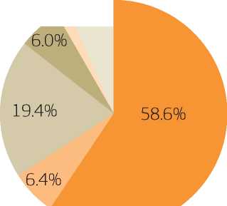
■ Value of time savings
■ Train operating costs savings
■ Vehicle operating costs savings (road)
■ Net fare revenues increase (rail-bus)
■ Accidents
Emissions
The main purpose of the sensitivity analysis is to determine the ‘critical' variables of the model. Such variables are those whose variations, positive or negative, have the greatest impact upon the project's economic results.125
The ‘critical' variables are conventionally considered those for which an absolute variation of 1 % gives rise to a corresponding variation of not less than 1 % in the ENPV - elasticity is unitary or greater.
|
VARIABLES |
Variation of ENPV + 1 % of variable -1 % of variable | |
|
Investment costs |
-1.01 % |
1.01 % |
|
Maintenance costs |
-0.02 % |
0.02 % |
|
Baseline traffic (without project) |
1.3 % |
-1.3 % |
|
Incremental traffic (induced by project) |
0.2 % |
-0.2 % |
|
Time savings |
1.03 % |
-1.03 % |
|
Savings of road VOC |
0.5 % |
-0.5 % |
|
Accident savings | ||
|
Externalities | ||
|
TOC savings |
0.10 % |
-0.10 % |
The variables identified as critical are thus (i) the traffic, (ii) the investment costs and (iii) the time savings. These three variables are taken further to the switching value calculation and risk analysis.
For each critical variable a switching value has been computed, i.e. the value for which the ENPV becomes zero, or in other words the maximum (negative) variation range over which the project would be still breaking-even economically. The results are summarized in the following table.
|
CRITICAL VARIABLES |
Value for which ENPV = 0 |
|
Investment cost |
137% |
|
Baseline traffic |
- 36% |
|
Time savings |
-110% |
The above values essentially confirm the economic case of the project is quite solid.
Although not very relevant for the financial indicators, given their highly negative profile, switching values were calculated for the FNPV(C) to show the variation range required to reach financial break-even.
|
CRITICAL VARIABLES |
Value for which FNPV(C) = 0 |
|
Investment cost |
-95% |
|
Revenues |
+ 1,816% |
|
O&M costs |
-4,067% |
The above results confirm the very negative financial profile of the project - which would require huge variations of the parameters - completely outside the realistic range - to reach break-even.
Risk analysis
Considering the particulars of the project, the following specific risks are considered.
Construction
The construction includes some technical challenges, e.g. replacement of existing tracks under railway operation, construction/ repair of 32 bridges, construction of 1.26 km of new tunnels. Works will require the employment of technical expertise and capacity, as well as proper co-ordination and supervision of activities.
Land acquisition
Land acquisition is an issue as the project includes some 26km of new alignment. However, the work plan (to be included in the tender documents) provides for a staged handing-over of the site, starting with the online sectors, whilst the expropriation procedure would be carried out in parallel. The procedure should be also eased by the recent new expropriation law.
Maintenance
Maintenance is a key issue for the long and short term sustainability of the investment. Regular maintenance is required in order to maintain the upgraded line in its design parameters (e.g. 160 km/h speed). Failure to ensure this would lead to speed restrictions which in turn would cancel out the benefits of the investment.
Demand
A traffic risk is inherent to any transport infrastructure project. This is equally true for the baseline traffic (without project) assumptions and for the incremental traffic (with project) forecasted.
The traffic risk also relates to the above factors as the improved level of service and efficiency gains for users (and in turn the demand reaction) depends on the operators' ability (both for passengers and freight) to exploit the potential provided by the improved infrastructure for enhancing the level of service provided.
The following matrix summarises the qualitative assessment of the above risks in terms of significance and probability of occurrence.
|
Risk |
Probability |
Impact |
Overall risk |
Mitigation measures |
Residual risk |
|
Construction risks |
D |
III |
High |
Contracting experienced supervision services; improving the staffing and training of PMU |
Medium |
|
Land acquisition |
D |
III |
High |
Staged handing-over of site starting with the online sections, in parallel with finalising land acquisition |
Low |
|
Operation -maintenance |
C |
III |
Medium |
Maintenance budget for the line to be increased, within a wider network reform programme |
Low |
|
Demand risk |
C |
IV |
High |
A parallel service improvement programme to be planned, including a more competitive passengers timetable, new rolling stock, etc. |
Medium |
Evaluation scale: Probability: A. Very Unlikely; B. Unlikely; C. About as likely as not; D. Likely; E. Very likely. Severity: I. No effect; II. Minor; III. Moderate; IV. Critical; V. Catastrophic.
Risk level: Low; Moderate; High; Unacceptable.
The project promoter will need to carefully assess the above risks and plan appropriate mitigation measures.
However, even with the assumed mitigation, the risk of construction cost overruns. In addition, the risk of time savings not actually materialising cannot be excluded, therefore a quantitative risk analysis was considered to add useful information.
Quantitative risk analysis
The quantitative risk analysis was performed using the following steps:
• assigning the probability distributions to the critical variables identified above;
• running a Monte Carlo simulation;
• interpreting the results.
Probability distribution
Since no studies have been performed in the country thus far concerning the distribution of variables such as investment costs, O&M expenses, traffic etc., the probability distributions of the critical variables have been assigned based on a review of the international literature and practice.
Construction costs
Flyvberg et al. (2003) has investigated cost overruns for 167 large-scale transport infrastructure projects. The tendency is clearly right skewed, where cost overruns are commonly occurring. In fact, an average of 20 % cost overrun among the 167 road projects is calculated with the worst project having a 223 % cost overrun and -33.6 % cost under-run.
Time savings
A triangular distribution with a minimum of -50 % of the variable, a most likely value of 0 % changes in estimated value and a maximum value of +5 % was assumed.
Baseline traffic
A Gauss profile distribution was assumed ranging from -50 % to +50 % with the mean of 0 % changes in estimated value.
The risk analysis has been performed with a specialised software for 5,000 simulations. The technique used is Monte Carlo simulation which involves a random sampling method of each different probability distribution selected for the actual model set-up. The three variables are considered independent of each other, so each ‘extraction' takes a random value for each variable to compute the corresponding ERR. The distribution of the ERRs obtained is presented below:
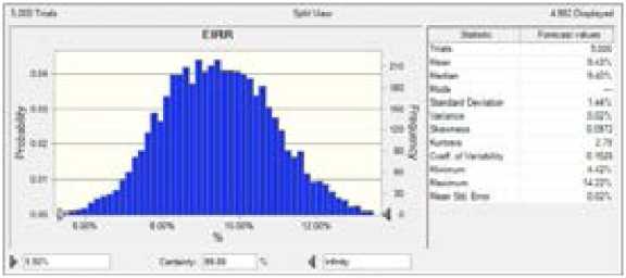
The above chart indicates that there is a 99.8 % probability for the ERR to be higher than 5.5 %, from a range of possible values starting from 4.4 % to 14.2 %.
The most likely value of ERR is 9.4 % with a standard deviation (quantifying the variation of the results from the expected value) of 1.4 %.
The results of the risk analysis clearly reconfirm the strong economic case of the project.
City X is a medium sized city of 300,000 inhabitants. The motorised mobility in the city is ensured by private transport as well as an extended bus network. The modal share in the city is 45 % public transport (bus) and 55 % individual transport.
The residential area Y, 7 km North-East of the city centre, is rapidly expanding. Mobility demand is increasing rapidly and the road connecting the residential area Y to the city centre/business area is heavily congested at peak hours. To ease this situation, the City Transport Authority is proposing to improve public transport connections to the city centre and implement a package of measures to promote public transport and encourage modal shift, including:
• Construction of 9 km of tram line (double track), with accompanying infrastructure (traffic signalling, traction infrastructure, necessary road works), as well as a new tram depot;
• Purchase of 15 new tram sets;
• Implementation of a Traffic Management System (TMS), including Passenger Information System at stops, integrated electronic ticketing, automatic vehicle location systems for public transport, public transport priority.
In addition, existing bus services in the area will be redefined with a feeder function to the new line. The public transport modal share is expected to improve, passing from the current 45 % to 47 %.
In this case study, time savings are expected in the transport system, due to the introduction of the new tram system and the reorganisation of the bus services, for the traffic diverted from the bus services and the individual cars to the tram. In addition, the impact of the shift to tram usage and the re-organisation of bus services will also translate into lower pollutants emissions from traffic, thus contributing to climate change mitigation126.
The institutional set up, in terms of relations between entities involved in project implementation and operations, is briefly described below. The implications of this institutional set-up for the analysis of cash flows, financial sustainability and assessment of State aid are duly taken into account in the rest of the analysis and will be highlighted when relevant in this case study127.
The City is the project beneficiary. As beneficiary, the City will receive the EU grant, and also draw a loan from an International Financing Institution (IFI) to co-finance the implementation of the project. In addition, it will co-finance the remaining part with own resources.
The City holds the strategic management of the public transport system through the Transport Authority, which is the budget unit of the City in charge of overall mobility policy128.
The City has entered a Public Service Contract (PSC) with the in-house Transport Operator. The PSC establishes the responsibilities, modalities for operation and compensations for public transport services. The contract is compliant with national and EU legislation regulating the provision of public service obligations129.
According to the PSC, the City will remain the owner of all the project assets (infrastructure, rolling stock and TMS), which will be made available for use to the public Transport Operator against payment of a lease. The City will also bear expenditures on replacements of project assets.
The Transport Operator holds the responsibility of operating and maintaining the project assets and bears all associated expenditures.
The general objective of the project is to ensure an efficient public transport service in the urbanised areas of the City. Specific objectives include:
• reducing road traffic congestion, accidents and negative environmental impacts, positively influencing the quality of urban life and the environment;
• improving the quality of the public transport travel experience, through increased quality standards;
• shortening travel time of public transport of vehicles and passengers without worsening traffic conditions.
As a secondary effect, it is expected that the project will also increase the attractiveness of the area around the planned investment through increased public transport availability.
The project objectives are in line with the national, regional and municipal strategies related to the overall territorial and spatial development as well as those related to the transport sector. In particular, the project responds to a priority defined in the City's multi-modal Mobility Plan, namely identifying needs and solutions for urban mobility. The objectives of the project are also coherent with the policies of the Commission on urban mobility130 and are well aligned with the objectives of the Operational Programme Transport. In particular, the project will contribute to the achievement of the following OP indicators:
|
Indicator |
OP 2023 target |
Project (% of OP target) |
|
Output indicators | ||
|
Total length of new or improved tram lines (km) |
32 |
8 (40 %) |
|
Result indicators | ||
|
Incremental number of passengers using urban public transport (M passengers/year) |
40 |
10 (25 %) |
In most transport projects different project options can generate different levels of traffic, so that a detailed definition of project options precedes the demand analysis estimating and forecasting the level of traffic for each of the project options.
The multi-modal Mobility Plan identified the need for improving the connections between residential area Y and the city centre as a priority, given the current heavily congested conditions and the foreseeable worsening of the traffic burden due to the fact that residential area Y is expanding.
In the Mobility Plan, a first screening of available options, with a multi-modal perspective, was done based on a Multi-Criteria Analysis (MCA). Selection criteria included technical feasibility, costs, environmental impacts and social acceptability131. Based on this screening, alternative project options such as the increase of road capacity by enlarging road infrastructure and the construction of an alternative road connecting the area Y and the city centre were discarded. The public transport option was considered the most effective and the number of alternatives was narrowed down to three, as follows.
• Option 1: strengthening of bus services with implementation of bus lanes and fleet renewal, as well as implementation of TMSs with public transport priority.
• Option 2: new tram line (7.5 km, along Alignment A running along the existing road) with tram rolling stock purchase, re-organisation of bus services with a feeder function, as well as implementation of TMSs with public transport priority.
• Option 3: new tram line (9 km, along Alignment B, mostly along the existing road, but with a small detour to allow another residential area along the way to be served) with tram rolling stock purchase, reorganisation of bus services with a feeder function, as well as implementation of TMSs with public transport priority.
The without-the-project (counterfactual) scenario, against which the project options are compared, assumes a continuation of business as usual, maintaining the level of expenditures which would guarantee the basic functionality of assets. This implies a slight worsening of the modal share of public transport.
In the feasibility study a full CBA on all three project options was performed. Traffic forecasting was done separately for each of the three options, and implications in terms of investment costs, O&M, renewals, as well as benefits, were assessed separately. Option 3 was selected as it scored the highest economic internal rate of return. This case study shows the CBA carried out for the selected option only.
The demand analysis is carried out based on a multi-modal network traffic model (traffic diagnostic and forecasting) owned by the City. The model is calibrated with data from the most recent comprehensive traffic study (the Transport Authority carries out traffic surveys every 5 years). Model results are used to inform both the financial and the economic analyses. Traffic forecasts were carried out separately for the without-the-project scenario and for each of the three project options. Forecasts were made for three years (year 4 - first full year of operations, year 15 and year 25) and linear interpolation was used to forecast the remaining years. This case study shows the traffic forecasts carried out for the selected option only.
It is assumed that the city is congested and with a high level of suburban living. The average trip length is 7 km for buses and trams and 8 km for cars, while the average speed is 14 km/h for buses and 20 km/h for cars in the scenario without-the-project; and 14.3 km/h for buses, 19 km/h for trams and 20 km/h for cars in the scenario with-the-project (unchanged, since it is assumed that possible congestion relief effects will be counterbalanced by the implementation of TMS with public transport priority).
The traffic, after the traffic stabilisation and the corresponding shifts following project completion, shows a moderate traffic growth rate of 2 % from the opening (year 4) to year 10, 1 % up to year 15 and no growth afterwards132. Demand data for the without-the-project scenario and for the selected option are summarised in the following table. All data are expressed in millions (m) passengers or passengers-hours (h) per year.
|
Year 1 (start of construction) |
Year 4 (first full year of operation) |
Year 10 |
Year 15 |
Year 25 | |
|
Without-the-project scenario | |||||
|
Passengers | |||||
|
Bus |
42.4 |
45.0 |
50.2 |
52.7 |
52.7 |
|
Trams |
- |
- |
- |
- |
- |
|
Private transport |
52.0 |
55.2 |
61.6 |
64.7 |
64.7 |
|
Passenger-h | |||||
|
Bus |
21.2 |
22.5 |
25.1 |
26.4 |
26.4 |
|
Trams |
- |
- |
- |
- |
- |
|
Private transport |
20.8 |
22.1 |
24.6 |
25.9 |
25.9 |
|
With-the-project scenario | |||||
|
Passengers | |||||
|
Bus |
42.4 |
37.0 |
41.3 |
43.4 |
43.4 |
|
Trams |
- |
10.0 |
11.2 |
11.7 |
11.7 |
|
Private transport |
52.0 |
53.7 |
59.9 |
62.9 |
62.9 |
|
Passenger-h | |||||
|
Bus |
21.2 |
18.1 |
20.2 |
21.2 |
21.2 |
|
Trams |
- |
3.7 |
T-1 'ST |
4.3 |
4.3 |
|
Private transport |
20.8 |
21.5 |
24.0 |
25.2 |
25.2 |
Based on the traffic model results, demand in the with-the-project scenario has been qualified as existing (i.e. passengers already travelling in the without-the-project scenario), diverted (i.e. passengers diverted from bus and private cars to tram) and generated (i.e. passengers who were not travelling in the without-the-project scenario). The model shows that, in the with-the-project scenario, the incremental traffic (tram) is diverted from bus for 80 % of the total, diverted from individual transport for 15 % and newly generated for 5 %.
The information on current transport supply and foreseeable changes as a consequence of the project is provided by the Transport Operator and is compliant with the provisions on transport production as laid out in the Public Service Contract signed between the Transport Authority and the Operator. The planned supply is also compliant with the assumptions of the traffic model.
The following table summarises the main information about the current and planned public transport supply (bus and trams) and the expected private transport production. All data are expressed in millions (m) vehicles-km per year.
|
Year 1 (start of construction) |
Year 4 (first year of operation) |
Year 10 |
Year 15 |
Year 25 | |
|
Without-the-project scenario | |||||
|
Bus |
9.6 |
9.6 |
9.6 |
9.6 |
9.6 |
|
Trams |
- |
- |
- |
- | |
|
Private transport |
346.4 |
368.0 |
410.4 |
431.3 |
431.3 |
|
With-the-project scenario | |||||
|
Bus |
9.6 |
8.0 |
8.0 |
8.0 |
8.0 |
|
Trams |
- |
1.0 |
1.0 |
1.0 |
1.0 |
|
Private transport |
346.4 |
358.0 |
399.2 |
419.6 |
419.6 |
Investment Cost
The total cost of the project is estimated at EUR 160 million net of VAT (EUR 197 million gross), based on tender prices (the tenders for the construction works and the rolling stock purchase have all been awarded).
|
Total project costs (A) |
Ineligible costs (B) |
Eligible costs (C)=(AHB) | |
|
Planning/design fees |
3.0 |
- |
3.0 |
|
Land purchase |
5.0 |
- |
5.0 |
|
Building and construction |
73.0 |
- |
73.0 |
|
Tram infrastructure (incl. tracks and traction) |
630 |
- |
63.0 |
|
Tram depot |
100 |
- |
100 |
|
Plant and machinery or equipment |
57.5 |
- |
57.5 |
|
Tram rolling stock |
37.5 |
- |
37.5 |
|
Traffic Management System |
200 |
- |
200 |
|
Contingencies |
14.5 |
- |
14.5 |
|
Technical assistance |
- |
- |
- |
|
Information and promotion |
0.3 |
- |
0.3 |
|
Contract supervision |
6.5 |
- |
6.5 |
|
Sub-TOTAL |
159.9 |
- |
159.9 |
|
VAT |
36.8 |
36.8 |
- |
|
TOTAL |
196.6 |
36.8 |
159.9 |
The beneficiary completed the land purchase procedures (EUR 5 million)133. Contract supervision is set at 5 % of construction and equipment expenditures (EUR 6.5 million).
Contingencies are set at 10 % of project cost, which seems reasonable given the type of project, its state of advancement (tender awarded, works not started yet) and the associated residual risks.
The unit cost per km of tram line constructed (double track) appears reasonable if benchmarked with that of similar projects in cities with comparable network conditions.
The unit cost of the tram rolling stock appears reasonable, taking into account the technical specifications of the rolling stock purchased.
Unit costs are specified below.
|
Investment component |
Unit cost |
Total cost |
|
Tram infrastructure (9 km) |
EUR 7 m/km (double track) |
EUR 63 m |
|
Tram rolling stock (15 tram sets) |
EUR 2.5 m/tram set |
EUR 37.5 m |
VAT is set at 23 % and is fully recoverable for the City under national legislation.134 For this reason, VAT is a non-eligible cost for the project.
The O&M costs are borne by the Transport Operator. The following O&M unit costs have been used in the analysis:
|
Project component |
O&M unit cost |
|
Tram (infrastructure* and rolling stock) |
EUR 6 /tram vehicle-km |
|
Bus rolling stock |
EUR 3/bus vehicle-km |
* Including tracks and overhead line system.
Unit costs include traction (including a yearly amount earmarked for replacement of overhead lines), maintenance and repair (including spare parts and excluding replacements), staff and other administrative costs (including the lease for the use of project assets).
No real growth of costs has been considered (see section 2.8.4 of the guide).
The impacts of different project components on the O&M have been assessed separately, taking into account O&M savings due to the reorganisation of the supply of bus services and the incremental O&M due to the new tram system. Savings due to reduction of the supply of bus veh-km do not counterbalance the increase of costs due to operating the new tram line and new rolling stock.
The project results in an overall increase in the O&M expenditures of EUR 1.2 million/year, resulting from additional O&M costs of EUR 6 million/ year for the tram system and a reduction of O&M costs of EUR 1.2 million/year for the bus system.
The necessary replacements of the new infrastructure, rolling stock and TMS have been considered during the reference period of the project (25 years), based on the economic life of the individual project assets, which were assumed to be as follows:
|
Investment component |
Economic life |
Replacement during reference period in % of initial investment |
|
Tram infrastructure |
30 years |
- |
|
Tram rolling stock |
20 years |
33 % every 10 years |
|
TMS |
8 years |
100 % |
Based on the provisions of the PSC, the replacement costs are borne by the City (project beneficiary)137.
The project does not generate net revenues (operating costs higher than operating revenues). The residual value of the investment is hence calculated based on the net book accounting method. The depreciation rates of the various investment components (taking into account the replacements) are as follows: 135
|
Investment component |
Depreciation rate |
|
Tram infrastructure |
3.5 % |
|
Tram rolling stock |
5.5 % |
|
TMS |
13 % |
Project revenues stem from user fares and, based on the existing institutional set-up, accrue to the Transport Operator. The public transport ticketing system is integrated between buses and trams.
The average ticket per passenger is EUR 0.33 /passenger, which in the first year of operations results in an incremental inflow of EUR 0.7 million. The pricing policy will not change, i.e. tariffs will remain at the same level with and without the project136. Traffic diverted from bus will not contribute to increase of revenues, since the users were already paying a ticket before. The increased revenues come from road users diverted to public transport and from generated users.
|
Unit |
Year 4 (first year of operation) |
Year 10 |
Year 15 |
Year 25 | |
|
Traffic diverted from road |
m EUR |
0.5 |
0.6 |
0.6 |
0.6 |
|
Generated traffic |
m EUR |
0.2 |
0.2 |
0.2 |
0.2 |
|
Total revenues |
m EUR |
0.7 |
0.7 |
0.8 |
0.8 |
The fare-box recovery ratio, i.e. the share of operating expenses recovered through user fares, is expected to be around 52 % in the first year of operations.
Compensations are provided by the Transport Authority to the Operator in the framework of the PSC. The contract is on a net basis, i.e. the Operator bears both the cost risk and the revenue risk. The Transport Authority pays compensations to the Transport Operator as a price per vehicle-km produced (bus and tram), net of the revenues collected from user fares137. The existing PSC has been found compliant with European Commission Regulations on the provisions of services of general economic interest, so that the operating State aid, if granted according to the PSC provisions, can be considered compatible with market rules138.
Compensations are not a cash flow in the consolidated financial analysis (inflow for the Operator, outflow for the Transport Authority). However, they will be used in the financial sustainability assessment.
The beneficiary negotiated a loan with an IFI of EUR 15 million. The conditions agreed for the loan include a maturity period of 15 years (including three years grace period during construction and 15 years for principal repayment, which starts in the first year of operation) and an interest rate of 3.5 % in real terms. The cash flows related to the debt service are used in the calculation of the financial return on national capital (FNPV(K)).
The financial and economic CBA is done in conformity with European and national guidelines for the preparation of the cost-benefit analysis of major investment projects.
The following key assumptions have been used in the analysis:
• the CBA is based on an incremental approach;
• the analysis consolidates cash flows between the Transport Authority (owner of all project assets and bearing replacement cost) and the Transport Operator (using project assets against payment of a lease and bearing O&M costs);
• contingencies are excluded from the financial and economic analyses and only considered in the assessment of the financial sustainability.
• the reference period for the analysis has been set at 25 years based on the average life of assets, including both implementation (three years) and operations (22 years);
• the financial and economic analyses are carried out at constant prices. For cash flows in real terms, a 4 % discount rate in real terms is used in the financial analysis and 5 % in the economic analysis;
• VAT is fully refundable under national legislation and therefore not eligible. Thus, the financial analysis is carried out on cash flows net of VAT;
• the residual value is calculated on the basis of the residual non-depreciated accounting value;
• the most recent macroeconomic forecasts were adopted, based on national statistics;
• the necessary expenditure on assets renewal has been properly recognised in the future project cash flows as operating costs, also for the purposes of the calculation of the pro-rata application of discounted net revenue..
The assessment of the PSC and the financial impacts of the project highlight compliance with European Commission Regulations on the provisions of services of general economic interest139 and that aid provided in the form of compensation to the in-house Transport Operator will remain a compatible State aid, thus not requiring notification to the European Commission's DG Competition.
Even if the project generates revenues paid by users (in the form of user fares), the project's net revenue (difference between the incremental operating revenues and O&M costs) is negative, which is why Article 61 of Regulation (EU) No 1303/2013 does not apply here.
EU GRANT
|
Calculation of Discounted Investment Cost (DIC) |
NPV 4% | ||||||||||||||||||
|
Investment cost (excluding contingencies) |
mEUR |
139.8 |
48.8 |
48.3 |
48.3 |
0.0 |
0.0 |
0.0 |
0.0 |
0.0 |
0.0 |
0.0 |
0.0 |
0.0 |
0.0 |
0.0 |
0.0 |
0.0 |
0.0 |
|
DIC / Investment cost cash-flow |
mEUR |
139.8 |
48.8 |
48.3 |
48.3 |
0.0 |
0.0 |
0.0 |
0.0 |
0.0 |
0.0 |
0.0 |
0.0 |
0.0 |
0.0 |
0.0 |
0.0 |
0.0 |
0.0 |
|
Calculation of Discounted Net Revenues (DNR) |
NPV 4% | ||||||||||||||||||
|
Revenue |
mEUR |
9.9 |
0.0 |
0.0 |
0.0 |
0.7 |
0.7 |
0.7 |
0.7 |
0.7 |
0.7 |
0.7 |
0.7 |
0.8 |
0.8 |
0.8 |
0.8 |
0.8 |
0.8 |
|
O&M cost |
mEUR |
-16.0 |
0.0 |
0.0 |
0.0 |
-1.2 |
-1.2 |
-1.2 |
-1.2 |
-1.2 |
-1.2 |
-1.2 |
-1.2 |
-1.2 |
-1.2 |
-1.2 |
-1.2 |
-1.2 |
-1.2 |
|
Replacement cost |
mEUR |
-38.6 |
0.0 |
0.0 |
0.0 |
0.0 |
0.0 |
0.0 |
0.0 |
0.0 |
0.0 |
-20.0 |
0.0 |
-12.5 |
0.0 |
0.0 |
0.0 |
0.0 |
0.0 |
|
Residual value of investments |
mEUR |
11.7 |
0.0 |
0.0 |
0.0 |
0.0 |
0.0 |
0.0 |
0.0 |
0.0 |
0.0 |
0.0 |
0.0 |
0.0 |
0.0 |
0.0 |
0.0 |
0.0 |
30.1 |
|
DNR / Net revenue cash-flow |
mEUR |
-33.0 |
0.0 |
0.0 |
0.0 |
-0.5 |
-0.5 |
-0.5 |
-0.5 |
-0.5 |
-0.5 |
-20.5 |
-0.5 |
-12.9 |
-0.4 |
-0.4 |
-0.4 |
-0.4 |
29.7 |
|
ELIGIBLE COST (EC) |
mEUR |
159.9 |
|
CO-FINANCING RATE OF PRIORITY AXIS (CF) |
85% | |
|
EU GRANT ( = EC x CF) |
mEUR |
135.9 |
|
1 |
2 |
3 |
4 |
5 |
6 |
7 |
8 |
9 |
10 |
11 |
12 |
13 |
14 |
15 |
20 |
25 |
|
Construction |
Operation | |||||||||||||||
In this case, the EU contribution has been calculated by multiplying the eligible costs shown in section IV above (EUR 159.9 million) by the co-financing rate of the relevant priority axis (85%), which results in an EU grant of EUR 135.9 million. In addition to the EU grant, the beneficiary will contract a loan of EUR 15 million and will contribute with own funds with EUR 45.7 million. The beneficiary will also ensure the pre-financing of the VAT (EUR 36.8 million), which is however recoverable. The financing structure of the project is described below:
|
Financing Sources |
m EUR |
% share |
|
EU grant |
135.9 |
69 % |
|
IFI loan |
15.0 |
8 % |
|
Project beneficiary’s contribution |
45.7 |
23 % |
|
of which VAT |
36.8 |
19 % |
|
Total |
196.6 |
100 % |
The financial profitability of the investment (as indicated by FNPV(C) and FNPV(K)) is negative, as expected for a project where project operating revenues are lower than the operating expenditures (including renewals and maintenance), which is typical in the urban public transport sector. The table that follows shows the results of the financial analysis.
|
12 3 |
4 5 6 7 8 9 10 11 12 13 14 15 20 25 |
|
Construction |
Operation |
|
Calculation of the Return on Investment |
NPV 4% | ||||||||||||||||||
|
Investment cost (excluding contingencies) |
mEUR |
-139.8 |
-48.8 |
-48.3 |
-48.3 |
0.0 |
0.0 |
0.0 |
0.0 |
0.0 |
0.0 |
0.0 |
0.0 |
0.0 |
0.0 |
0.0 |
0.0 |
0.0 |
0.0 |
|
Revenue |
mEUR |
9.9 |
0.0 |
0.0 |
0.0 |
0.7 |
0.7 |
0.7 |
0.7 |
0.7 |
0.7 |
0.7 |
0.7 |
0.8 |
0.8 |
0.8 |
0.8 |
0.8 |
0.8 |
|
O&M cost (including replacement cost) |
mEUR |
-54.6 |
0.0 |
0.0 |
0.0 |
-1.2 |
-1.2 |
-1.2 |
-1.2 |
-1.2 |
-1.2 |
-21.2 |
-1.2 |
-13.7 |
-1.2 |
-1.2 |
-1.2 |
-1.2 |
-1.2 |
|
Residual value of investments |
mEUR |
11.7 |
0.0 |
0.0 |
0.0 |
0.0 |
0.0 |
0.0 |
0.0 |
0.0 |
0.0 |
0.0 |
0.0 |
0.0 |
0.0 |
0.0 |
0.0 |
0.0 |
30.1 |
|
FNPV(C) - before EU grant / Net cash-flow |
mEUR |
-172.8 |
-48.8 |
-48.3 |
-48.3 |
-0.5 |
-0.5 |
-0.5 |
-0.5 |
-0.5 |
-0.5 |
-20.5 |
-0.5 |
-12.9 |
-0.4 |
-0.4 |
-0.4 |
-0.4 |
29.7 |
FRR(C) - before EU grant -12.26%
|
Verification of the Financial Sustainability of the Project | |
|
EU grant |
mEUR |
|
Project beneficiary's contribution to investment costs |
mEUR |
|
Project beneficiary's contribution to loan repayment |
mEUR |
|
Loan disbursement |
mEUR |
|
Revenues |
mEUR |
|
Incremental compensations under Public Service Contract |
mEUR |
|
Total cash inflows |
mEUR |
|
Investment cost (including contingencies) |
mEUR |
|
O&M cost (including replacement cost) |
mEUR |
|
Interest payments |
mEUR |
|
Principal repayments |
mEUR |
|
Total cash outflows |
mEUR |
|
Net cash-flow |
mEUR |
|
Cumulated net cash-flow |
mEUR |
|
45.3 |
45.3 |
45.3 |
0.0 |
0.0 |
0.0 |
0.0 |
0.0 |
0.0 |
0.0 |
0.0 |
0.0 |
0.0 |
0.0 |
0.0 |
0.0 |
0.0 |
|
3.4 |
2.8 |
2.8 |
0.0 |
0.0 |
0.0 |
0.0 |
0.0 |
0.0 |
0.0 |
0.0 |
0.0 |
0.0 |
0.0 |
0.0 |
0.0 |
0.0 |
|
0.0 |
0.2 |
0.4 |
1.3 |
1.3 |
1.3 |
1.3 |
1.3 |
1.3 |
1.3 |
1.3 |
1.3 |
1.3 |
1.3 |
1.3 |
0.0 |
0.0 |
|
5.0 |
5.0 |
5.0 |
0.0 |
0.0 |
0.0 |
0.0 |
0.0 |
0.0 |
0.0 |
0.0 |
0.0 |
0.0 |
0.0 |
0.0 |
0.0 |
0.0 |
|
0.0 |
0.0 |
0.0 |
0.7 |
0.7 |
0.7 |
0.7 |
0.7 |
0.7 |
0.7 |
0.7 |
0.8 |
0.8 |
0.8 |
0.8 |
0.8 |
0.8 |
|
0.0 |
0.0 |
0.0 |
0.5 |
0.5 |
0.5 |
0.5 |
0.5 |
0.5 |
20.5 |
0.5 |
12.9 |
0.4 |
0.4 |
0.4 |
0.4 |
0.4 |
|
53.7 |
53.3 |
53.5 |
2.5 |
2.5 |
2.5 |
2.5 |
2.5 |
2.5 |
22.5 |
2.5 |
15.0 |
2.5 |
2.5 |
2.5 |
1.2 |
1.2 |
|
-53.7 |
-53.1 |
-53.1 |
0.0 |
0.0 |
0.0 |
0.0 |
0.0 |
0.0 |
0.0 |
0.0 |
0.0 |
0.0 |
0.0 |
0.0 |
0.0 |
0.0 |
|
0.0 |
0.0 |
0.0 |
-1.2 |
-1.2 |
-1.2 |
-1.2 |
-1.2 |
-1.2 |
-21.2 |
-1.2 |
-13.7 |
-1.2 |
-1.2 |
-1.2 |
-1.2 |
-1.2 |
|
0.0 |
-0.2 |
-0.4 |
-0.5 |
-0.5 |
-0.5 |
-0.4 |
-0.4 |
-0.4 |
-0.3 |
-0.3 |
-0.3 |
-0.2 |
-0.2 |
-0.2 |
0.0 |
0.0 |
|
0.0 |
0.0 |
0.0 |
-0.8 |
-0.8 |
-0.8 |
-0.9 |
-0.9 |
-0.9 |
-1.0 |
-1.0 |
-1.0 |
-1.1 |
-1.1 |
-1.1 |
0.0 |
0.0 |
|
-53.7 |
-53.3 |
-53.5 |
-2.5 |
-2.5 |
-2.5 |
-2.5 |
-2.5 |
-2.5 |
-22.5 |
-2.5 |
-15.0 |
-2.5 |
-2.5 |
-2.5 |
-1.2 |
-1.2 |
|
0.0 |
0.0 |
0.0 |
0.0 |
0.0 |
0.0 |
0.0 |
0.0 |
0.0 |
0.0 |
0.0 |
0.0 |
0.0 |
0.0 |
0.0 |
0.0 |
0.0 |
|
0.0 |
0.0 |
0.0 |
0.0 |
0.0 |
0.0 |
0.0 |
0.0 |
0.0 |
0.0 |
0.0 |
0.0 |
0.0 |
0.0 |
0.0 |
0.0 |
0.0 |
i~r2~r3 4~r5~r6~r7~ts~t9T10Tii~ri2~r13T14T15T20T25
Construction Operation
FRR(K)
|
National Financing Sources | |
|
Project beneficiary's contribution to investment costs |
mEUR |
|
Loan |
mEUR |
|
Loan Balance | |
|
Beginning balance |
mEUR |
|
Loan disbursements |
mEUR |
|
Interest payments |
mEUR |
|
Principal repayments |
mEUR |
|
Ending balance |
mEUR |
|
3.4 |
2.8 |
2.8 |
0.0 |
0.0 |
0.0 |
0.0 |
0.0 |
0.0 |
0.0 |
0.0 |
0.0 |
0.0 |
0.0 |
0.0 |
0.0 |
0.0 |
|
5.0 |
5.0 |
5.0 |
0.0 |
0.0 |
0.0 |
0.0 |
0.0 |
0.0 |
0.0 |
0.0 |
0.0 |
0.0 |
0.0 |
0.0 |
0.0 |
0.0 |
|
0.0 |
5.0 |
10.0 |
15.0 |
14.2 |
13.4 |
12.6 |
11.7 |
10.8 |
9.9 |
9.0 |
8.0 |
6.9 |
5.9 |
4.8 |
-0.0 |
-0.0 |
|
5.0 |
5.0 |
5.0 |
0.0 |
0.0 |
0.0 |
0.0 |
0.0 |
0.0 |
0.0 |
0.0 |
0.0 |
0.0 |
0.0 |
0.0 |
0.0 |
0.0 |
|
0.0 |
0.2 |
0.4 |
0.5 |
0.5 |
0.5 |
0.4 |
0.4 |
0.4 |
0.3 |
0.3 |
0.3 |
0.2 |
0.2 |
0.2 |
0.0 |
0.0 |
|
0.0 |
0.0 |
0.0 |
0.8 |
0.8 |
0.8 |
0.9 |
0.9 |
0.9 |
1.0 |
1.0 |
1.0 |
1.1 |
1.1 |
1.1 |
0.0 |
0.0 |
|
5.0 |
10.0 |
15.0 |
14.2 |
13.4 |
12.6 |
11.7 |
10.8 |
9.9 |
9.0 |
8.0 |
6.9 |
5.9 |
4.8 |
3.6 |
-0.0 |
-0.0 |
|
Calculation of the Return on National Capital |
NPV 4% | ||||||||||||||||||
|
Project beneficiary's contribution to investment costs |
mEUR |
-8.7 |
-3.4 |
-2.8 |
-2.8 |
0.0 |
0.0 |
0.0 |
0.0 |
0.0 |
0.0 |
0.0 |
0.0 |
0.0 |
0.0 |
0.0 |
0.0 |
0.0 |
0.0 |
|
Interest payments |
mEUR |
-3.9 |
0.0 |
-0.2 |
-0.4 |
-0.5 |
-0.5 |
-0.5 |
-0.4 |
-0.4 |
-0.4 |
-0.3 |
-0.3 |
-0.3 |
-0.2 |
-0.2 |
-0.2 |
0.0 |
0.0 |
|
Principal repayments |
mEUR |
-10.0 |
0.0 |
0.0 |
0.0 |
-0.8 |
-0.8 |
-0.8 |
-0.9 |
-0.9 |
-0.9 |
-1.0 |
-1.0 |
-1.0 |
-1.1 |
-1.1 |
-1.1 |
0.0 |
0.0 |
|
O&M costs (incl. replacements) |
mEUR |
-54.6 |
0.0 |
0.0 |
0.0 |
-1.2 |
-1.2 |
-1.2 |
-1.2 |
-1.2 |
-1.2 |
-21.2 |
-1.2 |
-13.7 |
-1.2 |
-1.2 |
-1.2 |
-1.2 |
-1.2 |
|
Revenues |
mEUR |
9.9 |
0.0 |
0.0 |
0.0 |
0.7 |
0.7 |
0.7 |
0.7 |
0.7 |
0.7 |
0.7 |
0.7 |
0.8 |
0.8 |
0.8 |
0.8 |
0.8 |
0.8 |
|
Residual value of investments |
mEUR |
11.7 |
0.0 |
0.0 |
0.0 |
0.0 |
0.0 |
0.0 |
0.0 |
0.0 |
0.0 |
0.0 |
0.0 |
0.0 |
0.0 |
0.0 |
0.0 |
0.0 |
30.1 |
|
FNPV(K) - after EU grant / Net cash-flow |
mEUR |
-55.5 |
-3.4 |
-3.0 |
-3.2 |
-1.8 |
-1.8 |
-1.8 |
-1.8 |
-1.8 |
-1.8 |
-21.8 |
-1.8 |
-14.3 |
-1.7 |
-1.7 |
-1.7 |
-0.4 |
29.7 |
FRR(K) - after EU grant
-11.16%
The analysis of the financial sustainability at the project level aims to assess whether the project is able to balance out its positive and negative cash flows during the reference period. The analysis shows that the project implementation costs are covered by means of the EU grant, a loan and the beneficiary's own contribution. As can be expected for such projects, negative cash flows will be generated during project operations. In order for the project to be sustainable, the balance between inflows and outflows must be reached by means of increased compensation by the City within the framework of the PSC. As can be seen below, in its financial plans the city committed to increase compensation to the extent that it covers the expected operating losses of the transport operator, so that there is robust evidence that the financial sustainability of the project can be ensured.
FINANCIAL SUSTAINABILITY -PROJECT
1 12 1 3 4~r5~r6~r?~rs~r9~rio~r 11Ti2~r 15Ti4~ri5~r20T25
Construction Operation
The assessment of the financial sustainability of the project for the beneficiary aims to understand whether the City will have sufficient funds for financing the own capital contribution to project costs, the repayment of the loan and the planned amount of compensation in the framework of the PSC. The City of X explicitly allocated in the multi-annual financial forecasts a sufficient amount of funds to cover own contribution, including capital expenditures, the debt service for the project loan
and the pre-financing of the VAT140. In addition, the payment of yearly compensation under the PSC is explicitly mentioned as a long-term financial commitment in the multi-annual financial forecasts, with a specific yearly financial allocation. Under these conditions, the financial sustainability of the project for the beneficiary is secured.
The assessment of the financial sustainability of the project for the Transport Operator aims to understand whether the operator will have sufficient funds to operate the project asset, ensuring an adequate level of service and standard of maintenance. Total inflows and outflows for the Transport Operator after the implementation of the project have been compared and are shown in the table below.
1 2 3 4 5 6 7 8 9 10 11 12 13 14 15 20 25
Construction Operation
FINANCIAL SUSTAINABILITY -TRANSPORT OPERATOR
|
Verification of the Financial Sustainability of the Transport Operator | |
|
Revenue |
mEUR |
|
Compensations under Public Service Contract |
mEUR |
|
Total cash inflows |
mEUR |
|
O&M cost (excluding replacement cost) |
mEUR |
|
Total cash outflows |
mEUR |
|
Net cash-flow |
mEUR |
|
Cumulated net cash-flow |
mEUR |
|
14.0 |
14.3 |
14.6 |
15.5 |
15.8 |
16.1 |
16.5 |
16.8 |
17.1 |
17.3 |
17.5 |
17.6 |
17.8 |
18.0 |
18.2 |
18.2 |
18.2 |
|
14.8 |
14.5 |
14.2 |
14.5 |
14.2 |
13.9 |
13.5 |
13.2 |
12.9 |
12.7 |
12.5 |
12.4 |
12.2 |
12.0 |
11.8 |
11.8 |
11.8 |
|
28.8 |
28.8 |
28.8 |
30.0 |
30.0 |
30.0 |
30.0 |
30.0 |
30.0 |
30.0 |
30.0 |
30.0 |
30.0 |
30.0 |
30.0 |
30.0 |
30.0 |
|
-28.8 |
-28.8 |
-28.8 |
-30.0 |
-30.0 |
-30.0 |
-30.0 |
-30.0 |
-30.0 |
-30.0 |
-30.0 |
-30.0 |
-30.0 |
-30.0 |
-30.0 |
-30.0 |
-30.0 |
|
-28.8 |
-28.8 |
-28.8 |
-30.0 |
-30.0 |
-30.0 |
-30.0 |
-30.0 |
-30.0 |
-30.0 |
-30.0 |
-30.0 |
-30.0 |
-30.0 |
-30.0 |
-30.0 |
-30.0 |
|
0.0 |
0.0 |
0.0 |
0.0 |
0.0 |
0.0 |
0.0 |
0.0 |
0.0 |
0.0 |
0.0 |
0.0 |
0.0 |
0.0 |
0.0 |
0.0 |
0.0 |
|
0.0 |
0.0 |
0.0 |
0.0 |
0.0 |
0.0 |
0.0 |
0.0 |
0.0 |
0.0 |
0.0 |
0.0 |
0.0 |
0.0 |
0.0 |
0.0 |
0.0 |
Based on the assumptions made concerning the expected inflows and outflows, the table above clearly shows that the project operations will be sustainable for the Transport Operator thanks to the provision of compensation under the PSC. As described before, the inflow of operating compensation is reasonably secured in the long-term financial forecasts of the City. Under these conditions, the financial sustainability of the project for the Transport Operator is secured.
The socio-economic analysis includes the following impacts:
|
Costs (-) |
Benefits (+) |
|
Investment costs |
Consumer surplus: |
|
Replacements (paid by the City) |
- Travel time savings |
|
Producer surplus (-): |
- Vehicle operating costs savings (road users) |
|
- O&M (paid by the Transport Operator) |
- Fares |
|
- Fares |
Externalities |
|
- Operating costs (tram) |
- Accidents savings |
|
- Air pollution reduction | |
|
- Reduction of impact on climate change | |
|
- Noise impacts reduction |
Conversion factors were estimated based on national statistics on the average composition of project costs and shadow wage (for labour costs) and share of taxation (for energy costs). The correction factors are 0.9 for investment costs and 0.85 for O&M.
As described in section III on demand analysis, the multi-modal traffic model provides information on the generalised costs for users of public transport and individual cars, without and with the project. It is therefore possible to calculate the consumer surplus as the difference in generalised costs of the trip (including time savings and fares) for both existing traffic and traffic diverted from the origin mode (private car, bus) to the destination mode (tram). Benefits to generated traffic are calculated via the Rule of Half141. The main assumptions and parameters used for the calculation of the costs and benefits are summarised below.
Investment costs and replacements are included in the economic analysis at their economic value, i.e. conversion factors are applied to net financial cash flows to correct for the opportunity cost of labour142.
For the calculation of the producer surplus, the revenues accruing to the Operator have been compared to the Operator's O&M costs. In this case study, the producer surplus is negative and therefore a cost to the project, since the incremental revenues are lower than the incremental costs.
Travel time
Impacts on travel time are calculated based on the information provided by the traffic model on door-to-door travel time143.
The project results in an overall decrease in travel time in the transport system (reduction of passenger/h), mainly due to time savings for bus users and car drivers diverting to the newly introduced tram mode. In this project, existing car users remaining in the road mode will not experience time savings, since it is expected that the project will not generate any significant increase in road capacity (the possible reduction of road congestion and increase of car speed due to traffic diversion to tram will be counterbalanced by the limitation of road capacity due to the implementation of a new surface transport mode, such as the tramway, as well as the implementation of the Traffic Management System, heavily oriented towards the public transport priority).
The table below summarises the impact on travel time, in million passenger/h.
|
Year 4 (first year of operation) |
Year 10 |
Year 15 |
Year 20 |
Year 25 | |
|
Existing traffic |
-0.4 |
-0.4 |
-0.5 |
-0.5 |
-0.5 |
|
Bus |
-0.4 |
-0.4 |
-0.5 |
-0.5 |
-0.5 |
|
Private transport |
- |
- |
- |
- |
- |
|
Diverted traffic |
-1.1 |
-1.2 |
-1.3 |
-1.3 |
-1.3 |
|
Bus to tram |
-1.1 |
-1.2 |
-1.2 |
-1.2 |
-1.2 |
|
Private transport to tram |
0.0 |
-0.1 |
-0.1 |
-0.1 |
-0.1 |
|
Total |
-1.5 |
-1.7 |
-1.7 |
-1.7 |
-1.7 |
The following parameters have been adopted for the estimation of value of time:
|
Travel purpose |
Share of trips by travel purpose |
Value of time (EUR/h) | ||
|
Public transport |
Private transport |
Public transport |
Private transport | |
|
Work |
35 % |
45 % |
9 |
11 |
|
Non-work |
65 % |
55 % |
3.6 |
4.4 |
The cost saving approach has been adopted to estimate the unit VOT for work trips. Labour costs have been estimated based on national statistics. Unit VOT for non-work travel time has been calculated applying ratios respectively of 0.4 to work VOT. The share of trips by travel purposes is based on the most recent traffic surveys.
Unit values escalate over time with an elasticity of 0.7 to GDP growth per capita.
Vehicle operating costs savings (VOC)
The avoided VOC for the users switching from cars to public transport due to the project (diverted users) are counted as a benefit.
The adopted unit VOC is EUR 0.3 /car veh-km, based on national statistics and taking into account fuel costs (depending on road alignment and traffic conditions) and wear and tear of vehicles (oil, tyres, vehicle maintenance and depreciation). The unit VOC is applied to the amount of cars (vehicle-km) saved in the project option.
The VOC savings associated with the reorganisation of bus services (resulting in a reduction of the bus supply in vehicle-km) are accounted for in the Operator's O&M costs.
Benefits to generated traffic
The traffic model shows that 5 % of the incremental tram trips will be newly generated in the transport system. This will represent an increase of 2 % of the total motorised mobility in the city (including public and private transport).
The benefits to generated traffic have been estimated according to the Rule of Half144. The half of the generalised costs for existing users has been taken (including VOT and fares) and multiplied by the amount of generated users.
Accidents
The traffic diversion from cars to public transport is expected to reduce the number of accidents on the roads, via the reduction of distance travelled by road (reduction of vehicle-km).
The adopted probability of accidents, number of casualties, fatalities and injuries are taken from national studies and statistics.
Based on national statistics, the Value of Statistical Life (VOSL) has been estimated at EUR 400,000 per fatality and EUR 65,000 per injury. In addition, a value of EUR 13,500 per casualty has been estimated to cover direct medical and administrative costs associated with accidents.
Unit values escalate with GDP growth per capita, with an elasticity of 0.7.
Noise
Noise costs associated with the project have been estimated, taking into account the difference in noise levels due to transport activity related to tram, bus and individual cars. The number of people exposed to noise and the level of exposure with and without the project were assessed based on the noise maps produced during the environmental impact assessment. This estimation takes into account the type of noise source, the morphology of the territory, building patterns and the expected transport activity changes.
Based on the assessment, the project is expected to reduce overall noise levels. This, on the one hand, is due to the fact that the newly introduced tram mode will adopt anti-noise construction techniques on both the tram tracks and the trams, thus limiting noise emission and, on the other hand is due to the reduced level of traffic on roads (reduction of cars and buses).
The unit cost (EUR/year/person exposed) is identified based on national stated preference surveys and is related to the level of annoyance generated by a given level of sound emission and escalates with GDP growth per capita, with an elasticity of 0.7.
The differential noise cost is estimated multiplying the amount of persons exposed in the without and with-the-project scenario by the unit cost corresponding to the levels of noise in the without and with-the-project scenario.
Air pollution
A reduction of the environmental burden is expected due to traffic diversion from road-based modes (cars and buses) to trams, which generate a reduction of fuel consumption and hence lower air pollutant emissions. Tram operations are not expected to generate air pollution at the point of use. The indirect environmental impacts of the upstream process of energy production are taken into account in the assessment of climate change (see below).
It is assumed that there are national guidelines, based on clear assumptions and methodology, providing unit monetary costs of air pollution145 per vehicle-km, disaggregated by mode of transport and speed. In this case, the calculation of the impact was made based on the following steps146:
• quantification of the incremental transport production, in vehicle-km, by mode (tram, bus, individual transport);
• multiplication by a unit cost (EUR/vehicle-km).
The following monetary values per vehicle-km were taken into account for the calculation of air pollution impacts (based on national studies):
• for bus transport, EUR 0.37 /vehicle-km (for speed between 11 and 20 km/h, in urban area);
• for road transport, EUR 0.03 /vehicle-km (for speed between 21 and 30 km/h, in urban area).
Unit values escalate with GDP growth per capita, with an elasticity of 0.7.
Climate change
The variation of CO2 emissions due to the project is calculated, as well as its economic value.
Emissions for tramways, which are electrically powered, are assessed in relation to the upstream process of production of the required increase in electric energy. These emissions do not happen at the point of use of the tramway, but at the point of production of energy and depend on the national energy mix.
In summary, although a small increase of CO2 emissions is expected due to the increase of electricity consumption for tram operations (emissions related to energy production), the project will lead to an overall (incremental) reduction of CO2 emissions,
The calculation of the economic impact of CO2 emissions for road based modes was made based on the following steps:
• quantification of the incremental transport production, in vehicle-km, by mode;
• multiplication of the incremental vehicle-km by an emission factor (gCO2/v-km) to calculate the incremental emission of CO2;
• multiplication of the total amount of CO2 emitted by a unit cost (EUR/tonne);
The calculation of the economic impact of CO2 emissions for tramways was made based on the following steps:
• quantification of the marginal energy consumption (KWh/train-km);
• multiplication of the total incremental energy consumption (in KWh) by a national average emission factor (gCO2/KWh) to calculate the incremental emission of CO2;
• multiplication of the total amount of CO2 emitted by a unit cost (EUR/tonne).
The following emission factors were taken into account for the calculation of the economic impacts of CO2 emissions for road based modes and tramways (respectively, based on national studies and on international research):
• for bus transport, 1,133.2 gCO2/v-km (corresponding to a Euro III bus);
• for road transport, 347.4 gCO2/v-km (corresponding to Euro III 1.4 cc gasoline unleaded);
• for tram transport, 5 KWh/train-km and 496 gCO2/KWh (energy consumption per train-km and CO2 emissions per KWh depend on, respectively, project specific and country data).
The adopted unit costs per tonne of CO2 are in line with the ‘central' values suggested in the general part of this guide. Following the recommendations made in section 2.9.9, the 2010 value and the annual adders are first converted to constant 2013 prices and for the years beyond 2030, the adders are continued at the 2011 to 2030 rate.
The results of the economic analysis are described below:
|
12 3 |
4 5 6 7 8 9 10 11 12 13 14 15 20 25 |
|
Construction |
Operation |
|
Calculation of the Economic Rate of Return |
NPV 5% | ||||||||||||||||||
|
C1. Investment cost (excluding contingencies) |
mEUR |
-118.3 |
-43.4 |
-43.4 |
-43.4 |
0.0 |
0.0 |
0.0 |
0.0 |
0.0 |
0.0 |
0.0 |
0.0 |
0.0 |
0.0 |
0.0 |
0.0 |
0.0 |
0.0 |
|
C2. Replacements (City) |
mEUR |
-27.6 |
0.0 |
0.0 |
0.0 |
0.0 |
0.0 |
0.0 |
0.0 |
0.0 |
0.0 |
-17.0 |
0.0 |
-10.6 |
0.0 |
0.0 |
0.0 |
0.0 |
0.0 |
|
C3. Producer surplus (Transport Operator) |
mEUR |
-3.2 |
0.0 |
0.0 |
0.0 |
-0.4 |
-0.3 |
-0.3 |
-0.3 |
-0.3 |
-0.3 |
-0.3 |
-0.3 |
-0.3 |
-0.3 |
-0.3 |
-0.2 |
-0.2 |
-0.2 |
|
C3a. Fares |
mEUR |
8.4 |
0.0 |
0.0 |
0.0 |
0.7 |
0.7 |
0.7 |
0.7 |
0.7 |
0.7 |
0.7 |
0.7 |
0.8 |
0.8 |
0.8 |
0.8 |
0.8 |
0.8 |
|
C3b. O&M cost |
mEUR |
-11.6 |
0.0 |
0.0 |
0.0 |
-1.0 |
-1.0 |
-1.0 |
-1.0 |
-1.0 |
-1.0 |
-1.0 |
-1.0 |
-1.0 |
-1.0 |
-1.0 |
-1.0 |
-1.0 |
-1.0 |
|
C4. Residual value of investments |
mEUR |
8.0 |
0.0 |
0.0 |
0.0 |
0.0 |
0.0 |
0.0 |
0.0 |
0.0 |
0.0 |
0.0 |
0.0 |
0.0 |
0.0 |
0.0 |
0.0 |
0.0 |
27.1 |
|
Total economic costs (C1 + C2+C3+C4) |
mEUR |
-141.1 |
-43.4 |
-43.4 |
-43.4 |
-0.4 |
-0.3 |
-0.3 |
-0.3 |
-0.3 |
-0.3 |
-17.3 |
-0.3 |
-10.9 |
-0.3 |
-0.3 |
-0.2 |
-0.2 |
26.8 |
|
Consumer surplus | |||||||||||||||||||
|
B1. Value of time |
mEUR |
115.2 |
0.0 |
0.0 |
0.0 |
8.3 |
8.5 |
8.8 |
9.0 |
9.3 |
9.6 |
9.8 |
10.0 |
10.2 |
10.4 |
10.6 |
10.9 |
11.4 |
12.1 |
|
B2. Vehicle Operating Costs (individual transport) |
mEUR |
40.7 |
0.0 |
0.0 |
0.0 |
3.2 |
3.3 |
3.3 |
3.4 |
3.5 |
3.5 |
3.6 |
3.6 |
3.6 |
3.7 |
3.7 |
3.8 |
3.8 |
3.8 |
|
B3. Fares |
mEUR |
-8.4 |
0.0 |
0.0 |
0.0 |
-0.7 |
-0.7 |
-0.7 |
-0.7 |
-0.7 |
-0.7 |
-0.7 |
-0.7 |
-0.8 |
-0.8 |
-0.8 |
-0.8 |
-0.8 |
-0.8 |
|
B4. Benefits to generated traffic |
mEUR |
23.0 |
0.0 |
0.0 |
0.0 |
1.7 |
1.7 |
1.8 |
1.8 |
1.9 |
1.9 |
2.0 |
2.0 |
2.0 |
2.1 |
2.1 |
2.2 |
2.3 |
2.4 |
|
Externalities | |||||||||||||||||||
|
B5. Accidents |
mEUR |
2.8 |
0.0 |
0.0 |
0.0 |
0.2 |
0.2 |
0.2 |
0.2 |
0.2 |
0.2 |
0.2 |
0.2 |
0.3 |
0.3 |
0.3 |
0.3 |
0.3 |
0.3 |
|
B6. Environment |
mEUR |
12.9 |
0.0 |
0.0 |
0.0 |
1.0 |
1.0 |
1.0 |
1.0 |
1.1 |
1.1 |
1.1 |
1.1 |
1.1 |
1.1 |
1.2 |
1.2 |
1.3 |
1.3 |
|
B6a. Air pollution |
mEUR |
11.2 |
0.0 |
0.0 |
0.0 |
0.9 |
0.9 |
0.9 |
0.9 |
0.9 |
0.9 |
1.0 |
1.0 |
1.0 |
1.0 |
1.0 |
1.0 |
1.1 |
1.1 |
|
B6b. Climate change |
mEUR |
1.6 |
0.0 |
0.0 |
0.0 |
0.1 |
0.1 |
0.1 |
0.1 |
0.1 |
0.1 |
0.1 |
0.1 |
0.1 |
0.1 |
0.2 |
0.2 |
0.2 |
0.2 |
|
B7. Noise |
mEUR |
3.6 |
0.0 |
0.0 |
0.0 |
0.3 |
0.3 |
0.3 |
0.3 |
0.3 |
0.3 |
0.3 |
0.3 |
0.3 |
0.3 |
0.3 |
0.3 |
0.3 |
0.4 |
|
Total economic benefits (B1+B2+B3+B4+B5+B6+B7) |
mEUR |
189.8 |
0.0 |
0.0 |
0.0 |
13.9 |
14.3 |
14.7 |
15.1 |
15.5 |
16.0 |
16.2 |
16.5 |
16.8 |
17.2 |
17.5 |
17.8 |
18.6 |
19.4 |
|
ENPV / Net benefits |
mEUR |
48.7 |
-43.4 |
-43.4 |
-43.4 |
13.5 |
14.0 |
14.4 |
14.8 |
15.2 |
15.7 |
-1.0 |
16.3 |
6.0 |
16.9 |
17.2 |
17.5 |
18.3 |
46.3 |
ERR 8.3%
B/C RATIO 1.35
A sensitivity analysis of the economic and financial profitability was carried out in order to identify under which circumstances the project becomes, respectively, economically unprofitable, if any, or financially profitable, if any. The analysis is carried out using disaggregated variables (i.e. demand and prices separately) to better identify possible critical variables.
The sensitivity analysis was carried out for the following variables:
|
Sensitivity of financial profitability |
Sensitivity of economic profitability |
|
Investment costs |
Investment costs |
|
O&M unit costs |
O&M unit costs |
|
Traffic demand - incremental |
Traffic demand - incremental |
|
Revenues (unit tariff) |
Value of Time (unit cost) |
|
Vehicle operating costs (unit cost) | |
|
Air pollution (unit costs) | |
|
Climate change (CO2 emissions) (unit cost) | |
|
Accidents (unit costs) | |
|
Noise (unit cost) |
Critical variables are defined as critical if a 1% change leads to a change of FNPV/ENPV equal to or higher than 1% (elasticity higher than 1). The estimated elasticity of the ENPV and FNPV(C) with respect to a 1% increase of the critical project variables is shown in the table below:
|
Variable |
ENPV elasticity |
FNPV(C) elasticity |
|
Investment costs ±1% |
±2.8% |
-1.0% |
|
Traffic demand (incremental) ±1% |
±3.1% |
- |
|
Value of Time (unit cost) ±1% |
±2.8% |
- |
Based on the analysis, only investment costs were found to be critical for the sensitivity of financial profitability. Regarding sensitivity testing of the economic profitability, the following variables were found to be critical: incremental traffic demand, investment costs and unit Value of Time. Switching values are calculated as follows:
|
Variables |
Switching value (ENPV = 0) |
|
Investment costs |
+ 35% |
|
Traffic demand |
-32% |
|
Value of Time |
-36% |
Spider diagrams illustrating the elasticity (line gradients) and switching values (line intersection with X axis) for the above mentioned variables are depicted below.
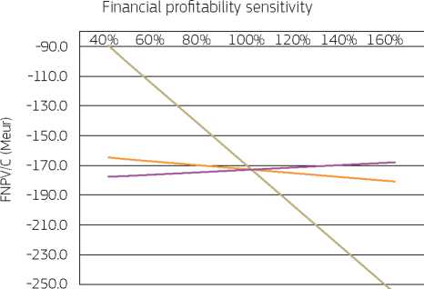
Change in the variable
— Investment cost
— O&M unit costs
— Traffic (incremental)
— Unit fare
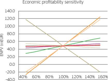
Change in the variable
— Investment cost
— O&M unit costs
— Traffic (incremental)
— Unit value of time
— Unit VOC
— Unit air pollution cost
— Unit climate change cost
— Unit accident cost
None of the above switching values seem to realistically threaten the assessment of the project financial and economic profitability. The risk analysis below analyses the main risk factors related to traffic forecasts and to investment costs, identifying the risk prevention/mitigation measures implemented (or to be implemented) by the beneficiary. Concerning VoT, a reduction of such an entity as to make the NPV null (-36%) is considered not realistic, given the macro-economic forecasts adopted for the project (it is here reminded that, in this case study, the VoT is calculated based on resource costs, i.e. labour cost).
A qualitative risk analysis has been carried out by the Beneficiary, with the aim to identify the main risks related to project implementation as well as operations. In addition, the main risk prevention and mitigation strategies are described.
|
Risk description |
Probability (P) |
Severity (S) |
Risk level (=P*S) |
Risk prevention / mitigation measures |
Residual risk |
|
Administrative risks | |||||
|
Problems with land purchase and acquisition of rights of way |
B |
II |
Low |
The need for land purchase is reduced to a minimum since the new line will mostly run on the existing road. The needed expropriation procedures are completed. Function in charge: Beneficiary. |
None |
|
Delays due to administrative procedures (permits, tenders, etc.) |
B |
II |
Low |
Establishment of a Project Implementation Unit with adequate resources within the Beneficiary structure, in charge of timely liaising with the relevant institutions/departments for timely finalisation of the needed procedures. Function in charge: Beneficiary. |
Low |
|
Late availability of EU grant co-financing |
B |
II |
Low |
Involve JASPERS technical assistance early in the project cycle. Negotiation of a loan available as of 1st year of construction Function in charge: managing authority and Beneficiary. |
Low |
|
Construction risks | |||||
|
Investment cost overrun |
C |
III |
Moderate |
Cost budget compared with relevant benchmarking to correct possible optimism bias. Publication of contract notices in the Official Journal of the EU to ensure wider competition. Selection of a professional external Construction Supervisor, with adequate budget. Function in charge: Beneficiary. |
Low |
|
Delays due to contractors (failure to meet contractual deadlines, withdrawal, bankruptcy, etc.). For rolling stock and equipment, this relates to both construction and provision. |
C |
III |
Moderate |
Selection of contractors in line with procurement legislation, including quality in the awarding criteria (not only lowest price). Close monitoring of contracts by PIU and by means of an external professional Construction Supervisor, with adequate budget. Function in charge: Beneficiary. |
Low |
|
Risk description |
Probability (P) |
Severity (S) |
Risk level (=P*S) |
Risk prevention / mitigation measures |
Residual risk |
|
Environmental and social risks | |||||
|
Impacts on air pollution, noise and climate change exceeding expectations. |
B |
III |
Moderate |
The environmental procedure has been completed according to high quality standards and can be reasonably considered comprehensive and complete. Mitigation Measures have been identified in the EIA, applying especially to the construction phase, and will be implemented by the Beneficiary. Function in charge: Beneficiary. |
Low |
|
Public opposition |
A |
II |
Low |
The public has been duly involved during the development of the EIA procedure and public notice has been given of all relevant decisions. Function in charge: Beneficiary |
Low |
|
Operational risks | |||||
|
Increase of operating costs higher than planned compensations, leading to liquidity problems for the operator |
B |
III |
Moderate |
The operating costs forecasts have been made based on the company historic costs as well as reasonable benchmarks, in order to reduce optimism bias. The PSC provisions are based on these forecasts, and provide for mechanisms of adjustment to changes of operating costs. Function in charge: Beneficiary and Operator in charge of ensuring correct functioning of PSC |
Low |
|
Significant shortfall in expected incremental public transport demand (implies lower benefits, lower revenues, need for higher compensations) |
B |
IV |
Moderate |
Adequate information and promotion measures to support modal shift. Conservative demand forecasts, also factoring in the impacts of the current economic downturn. Function in charge: Beneficiary. |
Low |
|
Transport supply not provided according to forecasted levels |
B |
III |
Moderate |
The Transport Authority and the Operator have signed a Public Service Contract, providing a clear framework for the provision of transport services, including planned production, quality standards and penalties for non-performance. In addition, the Operator is implementing management tools to monitor the quality of services and the level of user satisfaction (e.g. via user satisfaction surveys). Function in charge: Beneficiary (Transport Authority) |
Low |
Evaluation scale: Probability: A. Very Unlikely; B. Unlikely; C. About as likely as not; D. Likely; E. Very likely.
Severity: I. No effect; II. Minor; III. Moderate; IV Critical; V. Catastrophic.
Risk level: Low; Moderate; High; Unacceptable.
The results of the sensitivity and risk analyses indicate that the project overall risk level is low to moderate. The planned strategies to prevent the occurrence of the identified risks and/or mitigate their adverse impact are expected to bring project risk to a lower level. The residual project risks can be considered acceptable.
The flagship initiative for a resource-efficient Europe establishes the importance of using all types of natural resources efficiently and provides a general framework for policy actions for the European economy and environment for the next decade. Under the flagship initiative, a roadmap to a resource-efficient Europe was published in September 2011 defining the milestones to be met by 2020147.
In addition to the flagship initiative, a new Environment Action Programme (EAP) ‘Living well, within the limits of our planet' was adopted in November 2013 and will guide EU policy action on environment and climate policy for the next seven years. The aim is to guide Europe towards a resource-efficient, low-carbon and environmentally friendly economy in which natural capital is protected and enhanced, and citizens' health and well-being are safeguarded.
The implementation of this programme, however, will require the continued commitment of the Member States. In this respect, major projects supported by the ERDF and the Cohesion Fund can play a pivotal role in ‘protecting the environment and promoting resource efficiency' (thematic objective 6), as well as in ‘promoting adaptation to climate change, risk prevention and management' (thematic objective 5). The main expected areas of intervention for major projects are:
• water supply and sanitation;
• waste management;
• environment remediation, protection and risk prevention.
While being closely interrelated in many aspects, each sub-sector is characterised by different logics of intervention so that the Chapter is structured along these typologies of intervention, which are presented separately.
The EU water policy is largely based on the Water Framework Directive148 that sets up ambitious objectives for the quality and protection of all waters bodies (ecological status, quantitative status, chemical status and protected area objectives) and includes the key element of the River Basin Management Plans. The RBMPs provide the overall context for water management in a certain territory (the River Basin District, RBD) of the Union, including gaps, measures and objectives. In this respect the Cohesion Policy investments should take place within the context of the relevant RBMPs, including the preparation of programmes of measures at basin level, as well as within relevant implementation plans for the provision of particular services linked to other relevant EU water legislation (see box below).
In line with the results orientation of the new legislative framework of the cohesion policy, the principles for investments in the water sector are as follows:
• integrating the management of water resources on a river district scale. The river basin district' is the territorial unit basis for the management of water from all points of view and is defined as a set of terrestrial and marine areas, which include one or more neighbouring basins. In addition, water investments can be financed if River Basin Management Plans are adopted and are meeting minimum requirements set up in WFD (cf. thematic ex-ante conditionality 6.1, criterion 2);
• integrating economics into water management and water policy decision-making. To achieve its environmental objectives and promote integrated river basin management, the Water Framework Directive calls for the application of economic principles and requires an economic analysis of the different uses of resources and water services;
• polluter-pays principle151. The tariff policies for attaining the goal of economically and environmentally sustainable use of water resources must recover the cost of water services, including financial costs, environmental costs and resource costs, while taking into account social, economic and environmental effects of the recovery, as well as geographic and climatic conditions. In this regard, Member States are encouraged to define their pricing policy frameworks at national/ regional level;
• water efficiency152. Reducing water usage helps to preserve the available resources and prevent future droughts and also contributes to improving the competitiveness of an economy. It encompasses in particular water pricing providing incentives for users to use water resources efficiently, leakage reduction in distribution networks and, in areas where water deficit is structural, water reuse systems.
The following investment typologies are discussed in the rest of the section:
• renovation/development of infrastructure for water supply;
• renovation/development of infrastructure for wastewater collection and treatment.
Natural capital enhancing projects (e.g. green infrastructure) are not specifically treated in this section because usually associated to objectives of environment protection and ecosystem preservation (see section 4.3). However, in some cases, these projects can also achieve some of the water- (but also waste-) related benefits that are typical of the traditional engineering solutions. For example, preserving the Natura 2000 network is likely to have benefits ranging from regulating services, such as water resource savings, to cultural services, such as recreation. Vice-versa, development of infrastructure in the Integrated Water Supply service can also achieve benefits of environment preservation. That considered, both project typologies (i.e. infrastructure and natural capital investments) share the same methods for benefit evaluation. For this reason, the methodology presented below can be understood as a flexible framework for project appraisal, where a given benefit can be achieved through different investment types.
A selective list of policy and regulatory documents for the water sector is provided in the box below.
Blueprint to Safeguard Europe’s Water Resources
The Water Framework Directive (or Directive 2000/60/EC)
The Drinking Water Directive (or Directive 98/83/EC)
The Urban Waste Water Treatment Directive (or Directive 91/271/EEC)
The Bathing Water Directive (or Directive 2006/7/EC)
The Nitrates Directive (or Directive 91/676/EEC)
Directive 2008/105/EC on environmental quality standards in the field of water policy Directive 2009/54/EC on the exploitation and marketing of natural mineral waters Directive 2006/118/EC on the protection of groundwater against pollution and deterioration Directive 2001/83/EC on the Community code relating to medicinal products for human use Commission Staff Working Document ‘Climate Change and Water, Coasts and Marine Issues’ 149 150
For water projects, besides the traditional information in the socio-economic context, there are specific baseline features that
should be analysed more carefully when performing the context analysis:
• territorial planning framework. The project promoter should describe the existing national and regional sector policies (mainly for the use of water for human purposes, the treatment of sewage and the protection of water bodies elements) to ascertain the project's relevance. Also, clear and explicit links needs to be made between the water-related priorities in the operational programme and the relevant RMBPs;
• institutional context. Reference should be given to the institutional organisation of the water and sanitation services, including information on the capacity of the service provider (utility), the level of service integration, the role of the planning and/or control authority bodies, etc.;
• coverage and quality of the services in the area concerned by the project. The context analysis should describe: the current extension and population coverage of the water and wastewater systems151; levels of water consumption for civil, industrial, public and/or irrigation uses; level of physical and administrative water losses, both at production and in the distribution systems; reliability of the water supply and continuity of service; scarcity /abundance of the water sources; polluting loads on surface water bodies, including rivers, lakes, transition waters, estuaries and coastal seawaters;
• pricing policy. The project promoter should present the current pricing policy and level of charges paid by the users, as well as analysing the scope and implications of tariff increases or change in the pricing system following project implementation, taking into account considerations of equity linked to the relative prosperity of the Member State, or the region concerned.
Table 4.1 Presentation of the context. Water sector
|
Main information | |
|
Socio-economic trend |
- Population dynamics - National and regional GDP growth - Disposable income by population groups |
|
Environmental conditions |
- Reference to relevant river basin district - Current status of water bodies affected by the project, both as sources of water and as receptors of wastewater discharges - Planned qualitative and quantitative objectives on the status of the affected water bodies - Current amount of water drawn from natural sources and targets for future (increasing or decreasing) - Other uses, existing and planned, of the concerned water bodies: bathing, other recreational, productive uses, etc. |
|
General political, institutional and regulatory framework |
- Reference to EU directives and sector policy documents (see above) - Reference to national and regional strategies, including the River Basin Management Plans, any national implementation plan and accompanying programmes of measures - Reference to the priority axis and the interventions areas of the OP |
|
Water service institutional, regulatory and operational framework |
- Reference to the institutional organisation of the service: the level of the service integration, planning and/or control authority bodies, planning documents, etc. - Reference to the service control system - Reference to the operational organisation of the service and to the modes of supply - Service provider (utility): who will take over the operation and maintenance of the project infrastructure, and its capacity to implement (where relevant) and manage the infrastructure |
|
Main information | |
|
Existing service conditions |
- Service categories: drinking water, irrigation, industrial uses, sewers, wastewater treatment - Service catchment area (or areas) and population served - Specific water consumption and historic demand development by category of customers (domestic, public, industrial and others) - Connection rates, metering rate - Water physical losses and administrative losses - Infiltration to the sewerage network - Frequency and duration of water supply interruptions - Pricing policies and affordability ratios |
Source: Authors
The main general objectives of water investments are to increase the coverage or to improve the quality, effectiveness and efficiency of existing water supply and wastewater treatment services. Both logics of intervention can be driven by the need of the Member States to comply with the EU environmental acquis, as set out in the relative EU directives, but not exclusively.
The main motivations underlying the need for intervention are:
• increasing the number of households connected to centralised drinking water supply and/or wastewater networks152;
• improving the quality of drinking water;
• improving the quality of the surface water bodies and preserving ecosystems and biodiversity dependent on these surface water bodies;
• improving the reliability of the water sources and the water supply service;
• increasing efficiency in water production and/or distribution, e.g. through detection, measurement and reduction of water losses or management asset measures aimed at operating costs reduction;
• increasing efficiency in wastewater collection, removal, purification and elimination, e.g. with a strategy for disposal of sludge from urban wastewater treatment;
• replacing the use of water, preserving it from over-abstraction and/or providing for other efficient uses.
The scope is on investments in the Integrated Water Supply (IWS) service for civil, industrial and agricultural uses. The IWS segments include the supply and delivery of water as well as the collection, removal, purification and elimination of sewage. The re-utilisation of wastewater, while not strictly part of the IWS, is also discussed.
The following table provides some examples of IWS investments.
Table 4.2 Typical IWS investments
|
Examples | |
|
Renovation/development of infrastructure for drinking water supply |
- Construction of new infrastructures, e.g. aqueducts, intended to meet increasing needs - Completion of water supply networks that have been partially realised - Modernisation and/or replacement of the existing water pipes and of other elements of aqueduct (e.g. tanks, basins, spillways, pumping stations.) - Pressure zoning management intended to improve the efficiency of the water asset management |
|
Renovation/development of infrastructure for wastewater treatment |
- Replacement/extension of the sewage network (either combined or separate) - Construction /rehabilitation of wastewater treatment systems - Construction/rehabilitation of wastewater treatment plants with more stringent treatment for the reuse of water - Infrastructure for rainwater drainage |
Source: Authors
4.1.4.1 Factors influencing water demand
When forecasting demand for water, different factors need to be taken into account and duly analysed, including:
• demographic dynamics: the total water demand is directly related to the size of population. The project shall take into account the demographic forecasts and the migration flows for an estimate of the users;
• economic trend: even though in some cases there is relative or absolute decoupling between resource use and economic growth, a fast growing economy still generally demands a higher quantity of water than a flat or shrinking economy. In parallel, higher standards of living are associated with higher demand for water. If, within a given catchment area, tourism or production development is expected, it should be duly taken into account in forecasting the water demand;
• agricultural production trend: in the case of irrigation water, the demand depends upon the surfaces that are expected to be irrigated and the types of crops;
• industrial production trend: in the case of industrial use of the water or of industrial wastewaters, demand forecasting usually requires a specific analysis of the hydro-needs of the concerned production units, broken down by type of production;
• climate: demand for water has a seasonal component and climate change impacts may affect the availability of water in the long run;
• tariff system: it is important to consider the elasticity of demand with respect to tariffs. In some cases it will be necessary to estimate the elasticity for different income groups and also for small and large users, because it may have quite different values and distributive impacts. In any case, the elasticity of water demand with respect to service price should be estimated on a local basis. In fact this parameter varies considerably in different geographical areas that are otherwise similar.
4.1.4.2 Hypotheses, methods and input data
Demand is fundamentally made up of two elements:
• the number of users (civil use), the surfaces that will be irrigated subdivided by different kinds of crops (agricultural use) or the number and sectors of the production units which shall be served (industrial use);
• the quantity of water, that is being or will be supplied/treated for a given period of time.
The estimation of the demand curve may be based on data gained from the previous experience in the area involved or on published forecasting methods often based on the concept of the consumer's willingness to pay153. In case of replacements and/or completions, it is also useful to make reference to the data on historical consumption, provided that these data have been measured by reliable methods (for example from the readings of meter consumption).
The most important input data to be considered for forecasting the demand in water projects are:
• historical and current annual total and average consumption by type of consumers. The following categories of consumers are generally considered:
- household/commercial final consumers, residents and non-residents (i.e.: commuters, tourists, visitors for other reasons, etc.)154;
- industrial users;
- agricultural users.
• variability of seasonal and daily level of consumption (litres/day) to identify peak and off-peak demand.
4.1.4.3 Output of demand forecasting
The project promoter should provide projections related to volumes of water and wastewater that will be treated by the project and the polluting load that will be generated.
In general, a distinction between starting, potential and actual demand (or water resource and water consumption, respectively) can be made. The starting demand is given by the actual consumption before the intervention (see box below). The potential demand corresponds to the maximum requirement, which will be taken into account for the investment.155 The actual demand is the demand which is actually fulfilled by the investment in question and which corresponds to the expected consumption.
A first obvious evaluation criterion of the investment depends on the extent to which the actual demand may be close to the potential demand: the demand the investment can actually satisfy corresponds to the supply, net of any technical resource loss and release. Whenever the project may imply the use of water (surface or subsurface) resources, the actual availability of the resource flows required will be clearly shown by appropriate hydrological studies.
If the project involves the treatment and discharge of sewage, it is necessary to analyse the polluting load of the water that will be treated as well as the load capacity of the body intended to receive the polluting and nourishing substances, in a way that is compatible with environmental protection (Directive 2000/60/EC).
- Number of users served, broken down into main categories, and projections for future dynamics.
- Irrigated surface (hectares) by crop kinds.
- Number and type of production units served, as well as their water demand (including possible seasonal peaks) and expected wastewater production (including expected polluting loads).
- Water availability and demand per capita (l/d*inhabitant) or per hectare (l/d*hectare) or per production unit.
- Water quality data (laboratory analysis).
- Number of population equivalent, flow and peak rates, parameters of the polluting load of the water that will be treated (laboratory analysis) and quality constraints of the water that will be drained (defined by the law).
The implementation of any investment project should be justified against a set of feasible alternative options that would achieve the same objective(s). The analysis of options should be carried out separately for water and wastewater systems, plants and networks and shall be based on a comparison of:
• the possible strategic alternatives, for example: a dam or a system of crosspieces instead of a wells field or the agricultural re-utilisation of properly treated sewage; a central depurator instead of several local depurators; rehabilitation/ extension of existing treatment plants vs. new construction; re-lining against replacement, etc.;156
• the possible technical alternatives within the same infrastructure, for example: different location of wells, alternative routes for aqueducts or trunk lines; different building techniques for dams; different positioning and/or process technology for plants; utilisation of different energy sources for desalination plants, etc.
In selecting the options, the design alternatives must meet the requirements of the legislative framework (EU acquis) and, in particular, the European water policy (see above) and of the water sector programmes of the Member State. Options that respect both design alternatives and the policy constraints, will then be ranked and selected according to the methodology illustrated in section 2.7.2. In particular, to select the optimal option, a life-cycle cost approach must be adopted to assess all relevant costs over the lifetime of the project (investment costs, operational costs, maintenance costs, decommissioning costs and external costs)157.
4.1.6.1 Investment cost
In the case of IWS projects, the time horizon is typically 30 years (taking into account also the construction period). As regards to the technical life of equipment, which has an impact on the level of replacement costs that needs to be taken into consideration during the time horizon, it is recommended to split the assets into main broad asset categories, for instance:
• civil works (including operational buildings, reservoirs, access ways, etc.);
• pipes (including transport and distribution pipes, connections);
• electrical and mechanical equipment(including equipment built in wells, plants, pumping stations).
Assumptions on the technical life of the categories above need to be duly justified and presented in the CBA report.
4.1.6.2 Operation and Maintenance (O&M) costs
Typical operating costs items of water investments include energy, materials, services, technical and administrative personnel, maintenance, and sludge management costs. Projections of O&M costs shall be split into fixed and variable costs, and by category. In developing the O&M cost projections for both with and without the project scenarios, clear assumptions shall be made. In particular, the definition of the scenario without the project must be one of the operations based on a realistic estimate of the continuation of the service, as illustrated in the box below.
4.1.6.3 Revenues projections
The source of financial revenues in the IWS project comes from the application of charges to users for the services rendered, e.g. revenues for drinking water supply, drainage water collection and wastewater collection and treatment, sludge management, sale of purified water for industrial and agricultural purposes, etc.
The public/private water agencies/companies/entities that run the water management should, in the first instance, ensure the financial sustainability of the whole water management system, including investments in maintenance of infrastructure. Thus, adequate tariffs have to bet set up with the goal of ensuring an adequate level of recovery of the cost of providing the service, as well as financial sustainability of operations once the project is implemented, while at the same time respecting affordability constraints that might apply. When necessary, an affordability analysis must be carried out in line with the provisions outlined in Annex V.
The following approach is recommended for the incremental tariff to be considered in financial analysis:
• without the project: current tariffs should be set at a level of cost recovery of the existing system, therefore allowing for coverage of O&M, as well as depreciation of existing assets;
• with the project: tariffs shall be set at least to cover all financial costs, i.e. to cover O&M costs for the existing and new project assets, including depreciation and replacement of short-life all assets, starting from the ones with the shortest economic life158.
Note that for the purpose of the calculations, a unit tariff is usually calculated and applied, although in practice tariffs can be differentiated across user groups.
The counterfactual scenario is a realistic estimate of the continuation of the service as is, which could imply higher O&M costs than in the scenario with the project, or even cover some minor necessary investments (do-minimum), if estimated as needed.
Given the general rule, in the water and wastewater management sectors, the identification of an appropriate counterfactual can be complex. In case of projects that are motivated by the need to comply with the EU directives, business as usual would likely correspond to perpetuating a situation of infringement of EU and national legislations and environmental risk. Thus, the project promoter should, in principle, dismiss this scenario and adopt as counterfactual the ‘do-minimum’ solution.
In practice however, this approach is often not feasible. In fact, owing to technological constraints, it can be difficult to identify a technically viable minimum solution capable of reaching the stated objective, other than the project itself. In this case, the business-as-usual option should be considered an acceptable counterfactual, as the only technically feasible basis for comparison of costs and benefits. However, penalties for non-compliance with prevalent legislative requirements need to be projected, according to realistic and well-defined assumptions, and included in the financial analysis provided that are paid by the project promoter (while in economic analysis they are excluded to avoid benefits double counting).
IWS projects can produce different social benefits and costs, depending on the specific typology of project implemented as compared to the counterfactual scenario.
The main direct effects and externalities usually associated with the construction, modernisation and quality improvement of water supply and wastewater networks and/or treatment plants are summarised in the table below, together with the different valuation methods suggested.
Finally, a typical benefit that is not included below, because of a purely financial nature, are the O&M costs savings of the integrated water service, which, for some projects, can be the only aim of an asset management strategy.
Table 4.3 Typical benefits (costs) for water investments
|
Impacts |
Type |
Valuation method |
|
Increased availability of drinking water supply and/or sewer services |
Direct |
Averting behaviour Stated preferences (choice experiments) |
|
Improved reliability of water sources and water supply service |
Direct |
Averting behaviour Stated preferences (choice experiments) |
|
Improved quality of drinking water |
Direct |
Averting behaviour Stated preferences (choice experiments) |
|
Improved quality of surface water bodies and preservation of ecosystem services |
Direct |
Water bodies with a use value: market value, Averting behaviour, travel cost or benefit transfer Water bodies with a non-use value: contingent valuation or benefit transfer |
|
Resource cost savings (water preserved for other uses) |
Direct |
Long run marginal cost for water production |
|
Health impacts |
Externality |
Stated preferences Revealed preferences (hedonic wage method) Cost of illness |
|
Congestion savings due to improved rainwater drainage |
Externality |
Time savings |
|
Variation in GHG emissions |
Externality |
Shadow price of GHG emissions |
Source: Authors
In what follows, the above-mentioned listed benefits and the relative methods for evaluation are more extensively discussed.
4.1.7.1 Increased availability of drinking water supply and/or sewer services
Increased availability is typical direct effects of water and/or wastewater projects, which arises when new users are connected to the centralised water supply or sewer networks.
Given that water is a classic case of natural monopoly, where market prices are generally distorted, the preferred basis for benefit estimation is the users' willingness to pay (WTP) for the service. The WTP for being connected to the water supply/ sewerage service can be empirically estimated by applying the market prices of the best alternative technique feasible for the water supply/discharge of wastewater in the same catchment area (averting behaviour). In particular for the following projects:
• Water supply projects, the avoided capital and maintenance costs of self-provision of water, eg. by means of tank trucks, small-scale desalination plants (only for coastal areas), water wells or boreholes (especially for irrigation), can be applied. It is important to remark that these WTP refers to drinkable water, i.e. the underlying hypothesis is that the groundwater extracted with wells or borehole is drinkable. Otherwise, if purification is needed, additional costs for the purification process must be added;
• Sanitation projects, the avoided capital and maintenance costs of self-collection and discharge of wastewater, e.g. by means of closed tanks, can be applied.
To quantify the benefit, the WTP values (expressed in Euro/household) should be multiplied by the new households connected to the central network161.
Alternatively, stated preference methods (and in particular choice experiments - see Annex VI) can also be used to calculate users' WTP for the service rendered by the project. This is particularly the case of surveys being commissioned by water companies to provide evidence on what customers are willing to pay for improvements in customer service and environmental performance. WTP estimates are usually generated for attributes such as reduced frequency of service interruptions, improved taste and odour, reduced discolouration, improved pressure, and so on. Thus, the stated preference methods can be applied also to the benefits discussed below in sections 4.1.7.2 and 4.I.7.3.
4.1.7.2 Improved reliability of water sources and water supply service
This benefit arises when the methods for water abstraction, supply and distribution are improved so that the pressure of the water is increased (within prescribed limits), accidental service interruptions reduced and/or water supply shifts are eliminated.
As above, the WTP for improved reliability can be empirically estimated as the avoided cost of the inhabitants for a reliable self-provision (averting behaviour). For example, the costs avoided to be equipped with domestic tanks for collecting water and electric devices for pumping it into the house water systems with an adequate pressure.
These costs could include the investment costs for purchasing the tank and/or the pump (renewal), the costs of the electric power needed for its functioning, the maintenance costs and time spent by users (this includes time to collect information about hours and days of water rationing as well as the time spent to fill in the tanks and turning on/off the pumps).
4.1.7.3 Improved quality of drinking water
This benefit arises in case of interventions aimed at ensuring that the quality of drinking water supplied to citizens meets the minimum EU standards (see Drinking Water Directive).
When underground or surface water sources contain too high concentrations of chemicals or pollutants (e.g. iron, manganese, fluorine, etc.) water must be cleaned before supplying it to distribution system. Thus, drinking water quality can be improved with the construction, rehabilitation or upgrade of purification systems.
In the case of water quality being far from standards, purification treatments, can become more and more costly, as well as ineffective or, when intensive chemical processes are necessary to treat the highly polluted water, even health harming. In those cases, the quality of water can be improved working on the purification systems or even changing the water source (e.g. with the construction of aqueducts).
Again, the WTP for improved water quality can be empirically estimated as the avoided cost of the users to purchase good quality water on the market.162 For example, the avoided cost of purchasing water through tank lorries. Please note that this approach is pertinent to all users, including those that are connected to a centralised system. In fact, the best alternative technique for benefit estimation should consider a scenario where the existing supply is not compliant with the EU standards and is therefore interrupted and replaced.
Alternatively, the WTP can be estimated as the avoided cost to the users for setting up and operating domestic filtering systems that make water supply drinkable. The two approaches presented above are mutually exclusive.
In addition, positive heath impacts can be generated, as illustrated below in section 4.1.6.7. 159 160
4.1.7.4 Improved quality of surface water bodies and preservation of ecosystem services
The improvement of the surface water bodies' quality161 consists of reducing pollutant levels and/or increasing dissolved oxygen levels. In turn, this has the positive effect of preserving ecosystems and biodiversity dependent on these surface water bodies. Usually, this benefit originates from projects involving the extension of the wastewater treatment or the construction/rehabilitation of wastewater treatment plants (WWTPs) in compliance with EU requirements. Thanks to these projects, wastewater is treated before being discharged into the surface water bodies. The benefit can also arise, however, in case of projects dealing with removal of sludge and construction of wetland or projects concerning storm-water management facilities162, such as bio-retention systems, infiltration or retention basins.
Depending on the type of project under assessment, different methods can be adopted to estimate people's WTP to have surface water bodies of a better water quality. Indeed, the estimation of the WTP for a project aiming at improving the quality of a lake used for fishing differs from that of a lake used for bathing and differs also from that for a project concerning a river without any use. In other words, the use or non-use of the concerned surface water body must be known at first in order to choose the best estimation method.
• In case of water bodies (including seawaters) where prohibition to bathing, fishing or other recreational and/or productive activities is removed thanks to the project, an operational approach for benefit estimation is to use the market value of the concessions given for the provision of the recreational activities (e.g. beach resorts) or productive activities (e.g. fishing, shellfish) as proxy of WTP. In the absence of a market, the travel cost method to reach the facility or benefit transfer (see Annex V) can be used.
• In case of water bodies that are not used for bathing or other water related recreational and/or productive activities, the WTP for the simple existence (non-use value) of a less polluted water body (preserving or increasing the amenity of the place) must be estimated. A contingent valuation would be the preferred choice. However, it is usually expensive and time consuming (although nowadays, the progressive use of on-line panels of respondents is decreasing its cost). As alternative, a benefit transfer approach, transferring and adjusting values calculated somewhere else for similar projects, can be adopted.
Caution must be taken when defining the number of people to whom the concerned benefit must be applied. In principle, the WTP for improving the quality of water bodies with a use value should be multiplied by the number of persons who could potentially use the water body. Thus, a demand for the good should be carefully estimated.
Instead, the WTP for improving the quality of water bodies with non-use value should be multiplied by the total population of the catchment area, since the value reflects an existing or amenity value, i.e. what people are willing to pay just to keep an environmental asset in good quality. That said, often these values are space dependent, i.e. the non-use benefits received may decline with distance from the good or service. For example, in the case of a river, people may have higher non-use benefits for rivers closer to where they live than for similar rivers very far away. Hence, when aggregating non-use values, consideration could be given to the use of a distance-decay function. This issue shall also be discussed in sensitivity analysis.
4.1.7.5 Water preserved for other uses
The benefit of water preserved for other uses, current or future, arises first when interventions are aimed at reducing the water leaks of the distribution network. In other words, this is a typical benefit of water asset management projects: thanks to the reduced leaks, the volume of water needed to supply the network decreases and, as a consequence, an amount of water is preserved for other uses. Secondly, this benefit is generated when projects aim at avoiding the over-exploitation of a water source. For instance, when groundwater is replaced with water produced from other sources such as desalination or reuse of purified wastewater (more stringent treatment) for irrigation or industrial water supply. In contexts of water scarcity, this contributes to preserving the human environment and the whole biodiversity of the area.
The opportunity cost of the preserved water should be estimated on the basis of the long run marginal cost of production, reflecting the total social cost incurred to abstract an extra unit of water plus transportation cost from the source where it is abstracted to where it is used.
When the water tariff is well built (i.e. it reflects the long run marginal cost of production- see Annex III), the benefit is already captured by the operational cost savings of the operator which needs to use less groundwater to guarantee the same level of supply. If the tariff does not reflect the long run marginal cost, additional analysis is needed to measure the opportunity cost of the water preserved.
4.1.7.6 Health impacts
Positive impacts on health are mainly generated by two categories of projects:
• projects that improve the quality of drinking water owing to pollutant reduction, as measured by the difference between the contamination load carried by a unit volume of water, without and with the new system;
• projects that improve the effectiveness of the sewerage network and wastewater treatment, e.g. owing to avoidance of any contamination of the local aquifer with sludge.
Positive impacts on health should be included in economic analysis by attributing an economic value to the decreased morbidity rate for water-related diseases, taking care of possible benefit double counting with the WTP (see box).
The preferred method for the estimation of economic cost is, as usual, stated or revealed preference techniques based on the concept of willingness to pay/accept (i.e. either survey based techniques or the hedonic wage method).
In absence of this, the cost of illness approach, which combines direct and indirect costs into an overall societal estimate, can be adopted. Direct costs include the medical costs necessary for treating a particular disease (e.g. hospitalisation, medical supplies, rehabilitation care, diagnostic tests, drug prescriptions, etc.) and should be calculated on a case-by-case basis, depending on the type and severity of disease. Indirect costs measure the value of lost production because of reduced working time due to a particular illness. They are essentially calculated by multiplying the total period of absence (number of days) by the daily gross wage rate of the absent worker. In the case of children, disabled people and the elderly, the working days lost by their relatives (or to pay someone taking care of them) could be used as a proxy off the economic value for reducing the risk or the duration of illness.
In evaluating positive impacts in health, caution must be paid to avoid any benefit double counting with the WTP. For instance, if the defensive behaviour for bad drinking water quality of all consumers is to buy bottled water, it is unlikely that positive health impacts will be generated. Vice-versa, if consumers do not adopt a defensive behaviour and would still drink tap water in absence of the project, a WTP based on the avoided cost of purchasing water on the market is unrealistic, and the entire benefit will be the avoided cost of illness.163
That said, most likely, there will be situations in between, where consumers would drink both bottled and tap water and a combination of the two benefits apply. The project promoter should, however, consider realistic estimates of the volumes of water to which one or the other benefit is calculated. Accordingly, apply the WTP values only to a given share of the total water consumption and add the health benefit only for a realistic number of avoided cases (to be possibly estimated on the basis of hospital records).
4.1.7.7 Reduced congestion
When existing rainwater collection in urban systems is not capable of coping with rain water during hard rain, infrastructure to improve the drainage rate can be implemented, especially in light of the new challenges posed by climate change concerns.
Time saving is the most significant benefit that can arise from the improvement of a rainwater drainage system. Indeed, an improved rain water collection system leads to less congestion traffic and, in turn to time savings. For the estimation of this benefit please refer to the transport chapter. Obviously, this benefit is not related to interventions aimed at reducing the impact of hydrogeological disasters (that are dealt with in section 4.3).
4.1.7.8 Variation in GHG emissions
When relevant to the technical solutions envisaged in the project, the economic analysis will have to take into account the increase/decrease of GHG emissions as a result of:
• increased activities triggered by the project, including:
- sludge digesters, based on a quantification of gas production and related CO2 portion (to be justified in the technical feasibility study);
- sludge transport to disposal sites, based on quantification of dehydrated sludge and other waste from the WWTPs (screenings, grid) to be transported to a sanitary landfill and to surrounding agricultural fields;
• energy savings due to optimisation of the system.
Once quantified, the additional CO2 emissions generated or avoided should be monetised using the shadow price of CO2, as illustrated in section 2.9.9.
A sensitivity test of the results of both financial and economic analyses to changes in the value of the considered variables is highly recommended. Sensitivity analysis of water projects is advisable for both market-related variables and non-market goods. More specifically, the CBA results should be tested for changes of at least the following variables (when relevant for the project):
• assumptions on GDP trend
• demographic trend
• production trend, (when relevant)
• trend of unit water consumption
• number of years necessary for the realisation of the infrastructure
• investment costs (as disaggregated as possible)
• O&M costs (as disaggregated as possible)
• unit tariff or estimated WTP for water consumption
• WTP for increased coverage, increased reliability of supply, improved drinking water quality and/or quality of surface water bodies
• avoided cost of illness considered for the valuation of health benefits
• quantities and unit values of GHG emissions.
On this basis, a fully-fledged risk assessment must be carried out, typically, by assessing the risks presented in the following table.
Table 4.4 Typical risks in water projects
|
Stage |
Risk |
|
Regulatory |
- Unexpected political or regulatory factors affecting the water price |
|
Demand analysis |
- Water consumption lower than predicted - Connection rate to public sewage system lower than predicted |
|
Design |
- Inadequate surveys and investigation e.g. inaccurate hydrological predictions - Inadequate design cost estimates |
|
Administrative |
- Building or other permits/ Utility approvals/ Legal proceedings |
|
Land acquisition |
- Land costs higher than predicted - Procedural delays |
|
Procurement |
- Procedural delays |
|
Construction |
- Project cost overruns and/or delay in construction schedule - Contractor related (bankruptcy, lack of resources) |
|
Operational |
- Reliability of identified water sources (quantity/quality) - Maintenance and repair costs higher than predicted, accumulation of technical breakdowns |
|
Financial |
- Tariff increases slower than predicted - Tariff collection lower than predicted |
Source: Adapted from Annex III to the Implementing Regulation on application form and CBA methodology.
The EU legislation and policy on waste management are based on a series of principles which include the obligation to handle waste in a way that does not have a negative impact on the environment or human health, the encouragement to apply the priority order for waste management options in accordance with the waste hierarchy, the recovery of costs of waste management in accordance with the polluter pays principle and the principles of self-sufficiency and proximity.
These principles are central demands of the EU Waste Framework Directive164, which sets the basic concepts and definitions related to waste management.
According to the waste hierarchy, waste management strategies must aim primarily to prevent the generation of waste and to reduce its harmfulness. Where this is not possible, and waste is produced, priority should be first given to its preparation for re-use, then to recycling, then to other forms of recovery (e.g. in the form of energy in waste-to-energy facilities), and only as a final resort, waste should be disposed of safely in authorised, legally compliant landfills. Exceptionally, the Waste Framework Directive allows the departure from the hierarchy for specific waste streams where this is justified ‘by life-cycle thinking165 on the overall impacts of the generation and management of such waste' or based on the consideration of ‘general environmental protection principles of precaution and sustainability, technical feasibility and economic viability, protection of resources as well as the overall environmental, human health, economic and social impacts'.
The polluter-pays principle requires that the costs of waste management shall be borne by the original waste producer or by the current or previous waste holders.
For the programming period 2014-2020, the most important new policy development in this waste sector is the reinforced focus on resource efficiency, with the ultimate goal of making the most efficient use of the limited available resources (such as energy, water and raw materials), leading to cost cuts. Moving towards a more circular economy166 is essential to deliver the resource efficiency agenda established under the Europe 2020 Strategy for smart, sustainable and inclusive growth.167 Higher and sustained improvements of resource efficiency performance are within reach and can bring major economic benefits.
In addition, waste investments must be closely linked to the needs identified in the adopted waste management plans and waste prevention programmes in compliance with the Waste Framework Directive (cf. thematic ex-ante conditionality 6.2). A significant number of Member States still have important needs in terms of ensuring adequate management of solid municipal waste in compliance with EU standards, in particular to meet the 2020 target on preparation for re-use and recycling of certain materials from household waste and construction and demolition168 and the targets for the diversion of biodegradable waste from landfills169. In this respect, waste management will remain a priority for investments with ERDF and the Cohesion Fund.
A selective list of policy and regulatory documents for the waste sector is provided in the box below.
Waste Framework Directive (or Directive 2008/98/EC)
Regulation (EC) No 1013/2006 on shipments of waste Commission Decision 2000/532/EC on establishing a list of wastes
Council Directive 1999/31/EC on the landfill of waste Directive 2000/76/EC on the incineration of waste
Directive 94/62/EC of 20 December 1994 on packaging and packaging waste Directive 2012/19/EU on waste electrical and electronic equipment (WEEE) Directive 2013/56/EC on batteries and accumulators Directive 2000/53/EC on end-of-life vehicles
The baseline context elements recommended to be described for waste management projects are shown in the following table.
Table 4.5 Presentation of the context. Waste management sector
|
Main information | |
|
Socio-economic trend |
- Population dynamics - National and regional GDP and GDP per capita growth - Disposable household income by income groups |
|
General policy, and regulatory framework |
- EU directives and sector policy documents related to waste management (see above) - National and regional strategies related to waste management, including the Waste Management Strategies and Plans and the waste prevention programmes - Areas of intervention, objectives and specific targets of the operational programme and priority axis relevant to waste management |
|
Main information | |
|
Specific legal, institutional and operational framework for service provision |
- Institutional set-up of services, legal responsibilities for the planning, provision and control of waste management services, level of geographic integration, etc. - Control system of the service, including waste flow control - Operational organisation and forms of service provision and revenue collection, involvement of private sector in service provision, contractual arrangements including financial compensation - Level of taxes/fees/tariffs charged for services provided, level of cost recovery - Service provider(s) (utilities) in charge of service provision, operation and maintenance of the project infrastructure |
|
Coverage and quality of existing service provision |
- Service area and population served with service coverage rates - Quantities and composition of waste produced and collected at the local/regional level by source and type of waste (municipal waste from households, commerce, public parks and gardens, street waste, etc.) - Quantities and composition of waste imported from outside the local/regional level - Quantities of separately collected waste streams prepared for re-use or recycling (recyclable materials such as paper and cardboard, plastic, glass, metals), recovery or separate treatment or disposal (organics, bulky wastes, hazardous wastes, etc.) - Quantities of mixed residual wastes produced and collected and type of waste management methods implemented (for treatment and/or disposal) - Physical condition of existing facilities for waste treatment and disposal, risks for the environment from emissions of air, water and soil pollutants, extent of environmental damage to soil and groundwater, if any |
Source: Authors
The general objectives of waste management investments are usually the improvement of living conditions of the population and of environmental management in the local and regional context. The logic of intervention can be driven by the need of the Member States to comply with the EU environmental standards, as set out in the relative EU waste legislation, but not exclusively. Specific objectives involve:
• the development of a modern local and regional waste management system, to replace an inefficient and unsustainable waste management system based largely on landfills that are either non-compliant and/or reaching the end of their useful lifetime;
• increase of recovery of valuable materials and energy from waste, to reduce consumption of raw materials and fossil fuels;
• the reduction of health risks linked to an uncontrolled management and disposal of municipal and industrial waste;
• the curbing of raw material consumption and the planning of the final phases of material production and consumption cycles;
• the minimisation of GHG emissions and pollutants to air, water and soils from existing waste management facilities;
• replacement or technological overhaul of existing waste collection or treatment facilities, (e.g. refuse collection vehicles, waste incinerators) due to technological obsolescence.
The main types of waste management facilities are170:
• investments in facilities for the collection, temporary storage and/or transfer of waste (whether collected separately or not), such as municipal collection centres and waste transfer stations;
• material recovery facilities for preparation of (usually separately) collected materials for recycling;
• treatment facilities for separately collected biowaste (e.g. composting and anaerobic digestion plants);
• treatment facilities for mixed residual wastes from residential and non-residential sources (e.g. waste incinerators with energy recovery, mechanical-biological treatment plants, etc.);
• engineered landfills.
A map and a description of the technical characteristics of the proposed facility should be presented for a better comprehension of the local economic, social and environmental impacts of the project (see box).
- Basic data on waste to be treated: waste type (municipal waste, hazardous waste, packaging waste, biowaste) and annual quantity (t/y);
- Treatment processes with description of technologies used and individual design parameters (average and maximum throughput in t/d and t/h); specific consumption of energy, material and services consumed
- Mass balance of the treatment process with main inputs and outputs, including secondary raw materials recovered, energy produced (MWh of heat and/or power), mass losses.
- Physical features: area occupied by the plant (in thousand m2), covered and uncovered storage areas (in thousands m2), the distance from main agglomerations and discharge systems for effluent water and fumes.
- Information on procurement strategy and time-plan for construction
The implementation of any investment project should be justified against a set of feasible alternative options that would achieve the same objective (see section 6.2.5).
4.2.4.1 Factors influencing waste demand
When forecasting demand for waste management services, some key factors need to be taken into account and duly analysed, including:
• expected demographic growth and economic growth in relevant economic sectors;
• present and expected changes in national and European norms in waste management;
• evolution in the consumption habits and behaviour of waste producers, such as the increase in consumption correlated with the standard of living, the change in public attitude towards re-use and recycling activities or the adoption of clean products and clean technologies, with their potential consequences on waste streams, including the variation in the type of waste produced and the decrease or increase in waste production;
• technological, product and business model innovations: development of the circular economy, new business models (leasing, product service system, etc.) and product innovations are bringing major changes in the concept of ‘waste'/ ‘end-of-waste'.
4.2.4.2 Hypotheses, methods and input data
The demand for waste management services in the project area will be estimated based on the following input data: (i) current population and expected growth rate during the project horizon; (ii) current waste generation per capita and expected changes during the project horizon; and (iii) current waste composition and expected changes during the project horizon.
Other relevant aspects to be considered as part of the demand analysis (which will be also used for the identification and comparison of alternatives) are: (i) waste composition and calorific value; (ii) socio-economic conditions and geographic distribution of the customer base; (iii) potential market for waste sub-products (i.e.: recyclables and compost).
Demand is then forecasted from current waste generation levels taking into account demographic and industrial growth predictions; as well as the potential changes in waste producer behaviour.
The estimation of the demand, both in terms of quantity and quality of waste is a key factor in the identification of the project alternatives to define the type and capacity of the facilities that will be necessary to achieve the desired objective (see box in section 4.3.3).
The options analysis shall be carried out at two levels.
First, the analysis of the strategic global alternatives (e.g. different methods for waste management, different degrees of centralisation for waste treatment and disposal facilities) which shall be generally compared based on an economic analysis including externalities, where these differ notably between the individual options. In justified cases, other criteria related to technical, managerial and logistical aspects may be incorporated into the analysis.
Second, the analysis of the possible sites and more specific technical alternatives for the project, which shall be generally compared on the basis of costs and other criteria, including amongst others:
• efficiency of material recovery and/or production of energy (electricity and/or heat);
• actual market demand and off-take price for outputs (compost, recovered recyclable materials, residue-derived fuels, electricity and heat, etc.);
• public acceptance (i.e. chances of rejection by local communities and/or NGOs);
• hydro-geology (i.e. type of soil, stability of slopes, risk of flooding, risk of seismic movements, potential impact on water bodies and aquifers);
• accessibility (i.e. proximity and quality of access roads);
• ownership and zoning (i.e. land property and use);
• other factors (i.e. negative impact on residential areas and economic activities in surrounding areas).
In selecting the options, the design alternatives must meet the requirements of the legislative framework and, in particular, the EU Waste Framework Directive (Directive 2008/98/EC). Options that respect both design alternatives and the policy constraints, will then be ranked and selected according to the methodology illustrated in section 2.7.2. The box below provides some examples of options analysis at both strategic and technical levels.
- options analysis for the comparison of centralised and decentralised systems for the treatment of separately collected biowastes in a regional waste management system: one large centrally located plant vs. two or more smaller plants located closer to the main collection zones
- options analysis for the comparison of technological alternatives for the treatment of residual mixed waste collected (after separation of recyclables): mechanical-biological treatment with composting of the biological fraction vs. thermal treatment in a waste-to-energy facility
- options analysis for the identification of the economic optimal solution to further reduce mixed residual waste collected from an eminently rural area currently going to a landfill which is reaching the end of its useful lifetime (after achievement of targets for material recycling and landfilling of biodegradable waste at the regional level)
- options analysis for the comparison of different alternatives for transporting waste to a central treatment or disposal facility from distant collection zones: transport with or without a waste transfer station for the reloading of waste from small refuse collection vehicles to vehicles with larger payload and/or compaction
- options analysis for the comparison of different types of flue gas cleaning technologies in a waste-to-energy facility
- options analysis for the inclusion of automatised separation of different recyclable materials from mixed waste in the mechanical stage of mechanical-biological treatment plants and comparison of different systems available on the market
4.2.6.1 Investment cost
The time horizon for a project analysis is usually up to 30 years. In some cases, such as temporary storage waste facilities, collection centres or landfills, shorter values may be however used.
Typical investment costs of waste management projects include:
• civil works (including operational buildings, tanks, access ways, etc.)
• plant and machinery
• equipment and installations
• trucks for collection, (re)loading and transport of waste
• waste bins and containers
• technical assistance cost elements for ensuring proper behaviour from the waste producers (e.g. selection of waste, etc.)171
It is recommended to split the investment assets into main cost categories and assess their economic life separately. The economic life of some project assets can be shorter or longer than the adopted time horizon, in which case there will be a need for replacement or a residual value, respectively.
4.2.6.2 Operation and Maintenance costs
Projections of O&M costs shall be split into fixed and variable costs, with the latter in the form of unitary cost per tonne of waste going through each stage of waste management. Typical operating cost items of waste management investments are presented in Table 4.6.
Table 4.6 Typical O&M costs. Waste management sector
|
Main information | |
|
Variable costs |
- energy (electricity, heat) - fuels, materials and other consumables - emission fees (for emissions to air and water) - disposal of waste outputs produced in waste treatment facilities (only in case of projects dealing with individual components of a larger waste management system) - transportation costs |
|
Fixed costs |
- technical and administrative personnel - maintenance and repair - insurance - services |
Source: Authors
For certain facilities (such as landfills), closure costs and after-care costs following the closure of the facility, should be considered as well as part of the residual value at the end of the reference period. In developing the incremental O&M cost projections, clear assumptions shall be made for both with-project scenario and the counterfactual without-project scenario (either do-nothing or do-minimum). In particular, the choice of the counterfactual scenario follows the same logic as for IWS investments (see box in section 4.2.5.2 above).
It is expected that the technical feasibility study will establish the incremental cost per unit of produced waste on the basis of an analysis that takes into account the overall territorial integrated waste management system.
4.2.6.3 Revenues projections
The identification of revenues in waste management projects depends on the typology of investment, whether it addresses the entire waste cycle or just a segment of it. In the former case, typical sources of revenues are:
• the application of charges to users, either in the form of collection and disposal fees or taxes172;
• the sale of sub-products such as compost, recycled materials, refuse-derived fuel or solid-recovered fuel;
• the sale of the energy recovered such as heat and electricity, including, as the case may be, green certificates or bonuses for electricity produced from renewable waste fractions.
When the project concerns the entire waste management system, gate fees for individual waste management facilities are considered transfer costs between the different service providers (i.e. for waste collection, waste treatment, waste disposal in landfill) and therefore not included in the cash-flows. That is, gate fees are ultimately paid by the users and included in the user fees paid for waste management services.
On the contrary, if the project concerns only a segment of the waste management system (e.g. a waste-to-energy plant or a selection for recycling plant), a price for the service provided will be charged to the entities (municipalities, utilities, etc.) that ship the waste to be processed in the plant. Thus, gate fees shall be considered as the project revenues. Similarly, in case of recycled materials, if the aim of the project is to provide a service to third parties (e.g. to a consortium for the recycling of secondary raw materials), the revenue is calculated based on the price paid for the waste processing service and not on the sales price of the materials.173
Incremental fee/taxes charged to users shall be fixed at a level to recover the cost of providing the service, including replacement costs for the equipment with shorter lifespan, so as to ensure the overall financial sustainability of operations, while at the same time respecting affordability constraints that might apply. The definition of fees or taxes that are affordable for all customers does not imply that the same fee is applied to all. An affordability constraint for low income customers can be overcome with a tariff structure with lower rates for low income customers, and higher rates for the rest of the customers, including the non-residential ones (see Annex V).
Waste management projects can produce different social benefits and costs, depending on the specific typology of project implemented as compared to the counterfactual scenario. The main direct effects and externalities usually associated with the construction, modernisation and quality improvement of the integrated waste management are summarised in the table below, together with the different valuation methods suggested.
Table 4.7 Typical benefits (costs) for waste management investments
|
Impacts |
Type |
Valuation method |
|
Resource savings: avoided waste to landfill |
Direct effect |
LRMC of landfill disposal |
|
Resource savings: recovery of recyclable materials and production of compost |
Direct effect |
Market values/border prices/ LRMC |
|
Resource savings: energy recovery |
Direct effect |
LRMC of the substituted energy |
|
Visual disamenities, noise and odours |
Externality |
Hedonic price Stated preferences |
|
Variation in GHG emissions |
Externality |
Shadow price of GHG emissions |
|
Health and environmental hazards (variation in contamination of air, water and soils) |
Externality |
Shadow price of pollutants |
Source: Authors
In what follows, the above-mentioned benefits and the relative methods for evaluation are more extensively discussed.
4.2.7.1 Resource savings: avoided waste to landfill
For the purpose of the economic analysis of waste management projects, the reduction of the amount of waste finally
going to final disposal as a result of the project, which extends the economic life of the landfills, should be credited with an
economic value.
The data needed for benefit evaluation are:
• quantification of the volume (tonnes) of waste that is not going to the landfill for final disposal;
• unit economic cost. The cost of landfill disposal per tonne of waste varies depending on the size of the landfills, since there are significant economies of scale. Accordingly, the unit values adopted by the project promoter should be specific to the project context and consistent with the total annual waste generation in the project area that would otherwise go to the landfill. In the absence of project-specific data, some reference values of total cost per year of landfill disposal (taking into account both investment costs and operating and maintenance costs) depending on plant's capacity are provided in the study ‘Costs for Municipal Waste Management in the EU'174 (data should be updated to 2013 prices). 175
4.2.72 Resource savings: recovery of recyclable materials and production of compost
This benefit arises when the waste life-cycle closes, i.e. waste is used for making recycled products (e.g. plastic, glass and metals) or for the production of compost. In this case the resource recovered replaces the use of raw materials which, in turn, leads to cost savings from the societal point of view.
The economic value of the recovered recyclable materials and compost should be estimated at:
• the corresponding market price for the service rendered, if prices are assumed to reflect the opportunity cost of these products. Market prices should be justified along two dimensions:
- existence of an actual market for those products;
- consistency of the proposed prices with the existing market prices and comparable qualities for the sub-products.
• the corresponding border price for each sub-product, if market prices are assumed to be distorted. The information required for the calculation of conversion factors (CF) could be based on eco-industries data sets, or by national and international statistical offices or Customs.176
42.7.3 Resource savings: energy recovered
This benefit arises when the waste is used for producing energy in the form of electricity or heat. In other words, this benefit is associated with projects dealing with waste-to-energy plants, cogeneration plants and biogas plants (with production of fuel gas, electricity and/or heat). In this case, the energy recovered (using waste as source) replaces the use of energy from an alternative source/fuel (e.g. coal) which, in turn, leads to cost savings.
For the estimation of the avoided cost thanks to the substitution of the energy source/fuel, please refer to the methodology presented in section 5.7.4 of the energy chapter.
In the case of the substituted source being fossil fuel, an additional benefit related to displaced GHG emissions through energy generation from clean sources is generated (see section 4.3.6.6 below).
4.2.7.4 Visual disamenities, noise and odours
The negative externalities usually associated with waste management installations consist of visual disamenities, noise and odours. The negative impact of a landfill site, a waste incinerator or another major waste facility in terms or disamenities is normally a fixed amount that does not vary significantly with the amount of waste being disposed of or treated at the site but that depends on the mere existence of the waste facility at the site.
Depending on the typology of investment, these negative externalities can be either reduced or increased. Several methods are proposed in the literature to value in monetary terms these effects, ranging from revealed preferences (hedonic price method based on the market values of real estates) to stated preferences (WTP or WTA estimated via survey-based approaches).
The proposed approach of this guide for the estimation of the reduction/increase of visual disamenities, noise and odours is the hedonic price method. The underlying concept is that the proximity to a waste site causes a decrease in the value of the surrounding properties and, vice-versa, the closing of an existing site has the opposite effect.
For benefit quantification, the following steps should be carried out:
• first, it is necessary to fix the maximum territorial scope of the effect (or, in other words, to define the ‘affected area'). It is suggested to establish the maximum distance from the site perimeter for the effects to unfold on a case-by-case basis, depending on the characteristics and size of the waste facility and the urban structure around the site177;
• second, the surface and market value of the existing real estates in the affected area shall be estimated on the basis of land register;
• third, real estate price reduction (increase) should be calculated by looking at the land register value of real estates in similar zones that are (not) affected by a dump site178;
• finally, the following simplified formula179 can be applied in order to obtain the value of the benefit:
B = ZfS|*Vi* A%
• where: i is the type of property; S is the total surface of properties i (in m2); V is the observed value of properties (in Euro/m2); A% is the expected percentage increase/decrease in price because of the project.
• The result (B) is the estimated increase/decrease in property values as a result of a project.
4.2.7.5 GHG emissions
A reduction of GHG emissions is achieved when waste is: i) treated to reduce and stabilise the biodegradable components before being properly disposed, ii) recovered in form or materials which are sent to recycling, and/or iii) used for energy generation in substitution of fossil fuels180. In the first case, the decrease of GHG emissions, mainly methane (CH4), originates from the diversion of untreated biodegradable waste from landfills. In the second, materials recovered from waste enable savings in GHG emissions that would have resulted from the extraction and processing of raw materials. In the third, the waste-to-energy and co-generation (e.g. biogas) plants enable a reduction in GHG emissions that would have been produced by the alternative energy source.
The method suggested to monetise the saved GHG emissions from waste management projects consists of multiplying the amount of emissions avoided (expressed in CO2-equivalents per year, see below) by their unit economic costs.
The quantification of GHG emissions avoided due to treatment and proper disposal of waste should be based on the following.
• Specific emission factors for the waste management facilities (expressed in tonnes GHG/tonnes of waste throughput), multiplied by the amount of waste treated (in tonnes of waste throughput per year). By comparing the situations with the project and the counterfactual scenario181, it is possible to estimate the emissions change attributable to the project. The calculation of the specific emission factors will however require the knowledge or estimation of the average composition of the waste treated182;
• specific emission factors for the electricity and heat sources displaced by the project (in tonnes of CO2 per MWh produced), multiplied by the amount of energy produced [in gigajoules (GJ) or megawatts (MWh) produced per year];
• specific emissions avoided through recycling of materials recovered by the project183 (in CO2 per tonne of material recycled) multiplied by the amount of material recovered from waste sent to recycling (in tonnes per year).
In the absence of project-specific emission factors for the waste management facilities, average default emission factors can be derived from literature. For example, the ‘EMEP/EEA air pollutant emission inventory guidebook' provides guidance for the estimation of emissions for all major waste management practices.
In the case of avoidance of emissions due to energy recovery, the quantification of the volumes avoided follows the same logic illustrated below, in section 5.7.6 of the energy chapter. Generally speaking, CO2 emissions in the generation of electricity depends on the fuel and the efficiency of the facility used for electricity generation and ranges from 0.40 kg CO2/ kWh in the case of Combine Cycle Turbines (CCGT) to 0.95 kg CO2/kWh in the case of coal. Similarly, CO2 emissions in the generation of heat also depends on the fuel and the generation efficiency of the facility used for heat production and ranges from 0.27 kg CO2/kWh in the case of gas boilers to 0.45 kg CO2/kWh in the case of electric heating.
In order to evaluate the cost of CH4 emissions, the tonnes of CH4 emitted have to be converted into CO2-equivalents and then monetised following the instructions provided in Chapter 2, section 2.9.9.
42.7.6 Health and environmental hazards
The treatment of municipal solid waste produces emissions of specific pollutants into the air, water and soil.
For waste incineration, the main conventional pollutants emitted to the air are NOx, SO2, ozone precursors, particulates, heavy metals and dioxins. Such emissions are minimised through efficient flue gas cleaning systems that remove particulates and pollutant gases before the remaining flue gas is emitted to the air via the smokestack. Solid residues from waste incineration and flue gas treatment (including slag and bottom ash, fly ash and air pollution control residues) are disposed of at proper disposal sites, partially as hazardous waste. The flue gas cleaning processes may also give rise to emissions to water through wastewaters produced. These emissions are controlled using various physical-chemical wastewater treatment processes, which produce a filter cake which is disposed as hazardous waste.
For waste landfills, in addition to volatile organic compounds and dioxins, leachate is generated and emitted to the surrounding soil and water. Impacts related to the emission of leachate to the soil include the migration of contaminants to groundwater and/or surface water, where they can affect human health and the ecosystem. At compliant, engineered landfill sites, emissions to the soil are minimised through effective leachate collection and treatment systems.
Following the same logic of the reduction of GHG emissions, a reduction of emission of pollutants to the air, water and soil is achieved by implementing modern waste management systems. The recovery of energy in the form of heat and/or electricity from waste also reduces emissions of air pollutants from other energy sources that use fossil fuels.
To estimate the external cost of pollutant emissions, the usual approach consisting of quantifying the emissions avoided thanks to the project (measured in kg per tonne of waste) and valuing them with a unit economic cost (measured in euro per kg emission) applies.
Regarding the quantification stage, pollution pathways of emission are very project specific; they depend on a large number of variables including the quality of the recipient body (soil or water), the specific location of the plant, the technology used, the measures adopted for soil protection, etc. Thus, they should be calculated case by case with default emission factors being hardly usable or even not existing.
Regarding the valuation stage, most of the available information in the economic literature is on the marginal cost of air emissions and less information exists on the emissions cost to soil and water. Focussing on air emissions, the same sources mentioned in the transport chapter can be taken as reference (see section 3.7.6). As alternative, the Commission's Impact Assessment on the review of the National Emission Ceilings Directive184 can be used to value the external costs of health impacts, crop yield loss and damage to buildings owing to air pollution.
Sensitivity tests of the results of both financial and economic analyses to changes in the value of the considered variables is mandatory. Sensitivity analysis of solid waste projects is advisable for both market-related variables and the value of non-market goods. More specifically, the CBA results should be tested for changes at least of the following variables (when relevant for the project):
• assumptions on GDP trend
• demographic trend
• waste composition (e.g. possible reduction of the calorific value)
• number of years necessary for the realisation of the infrastructure
• investment costs (as disaggregated as possible)
• O&M costs (as disaggregated as possible)
• unit fee for waste collection and disposal or unit price for waste treatment service
• (avoided) cost of landfill disposal
• unit price of sub-products or of selection service
• fuel and energy prices
• quantities and shadow prices assumed for GHG emissions
• quantities and shadow prices assumed for pollutant emissions.
On this basis, a risk assessment must be carried out, typically, by assessing the risks presented in the following table.
Table 4.8 Typical risks in waste management projects
|
Stage |
Risk |
|
Regulatory |
- Changes of environmental requirements, economic and regulatory instruments (i.e. introduction of landfill taxes, bans on landfilling) |
|
Demand |
- Waste generation lower than predicted - Waste flow control/delivery insufficient |
|
Design |
- Inadequate surveys and investigation - Choice of unsuitable technology - Inadequate design cost estimates |
|
Administrative |
- Building or other permits - Utility approvals |
|
Land acquisition |
- Land costs higher than predicted - Procedural delays |
|
Procurement |
- Procedural delays |
|
Construction |
- Project cost overruns - Delay in construction schedule - Contractor related (bankruptcy, lack of resources) |
|
Operational |
- Waste composition other than predicted or having unexpectedly large variations - Maintenance and repair costs higher than predicted, accumulation of technical breakdowns - Process outputs fail to meet quality targets - Failure to meet limits of emissions produced by the facility (to air and/or water) |
|
Financial |
- Tariff increases slower than predicted - Tariff collection lower than predicted |
|
Other |
- Public opposition |
Source: Adapted from Annex III to the Implementing Regulation on application form and CBA methodology.
As specified in Article 9(5-6)(Thematic objectives) of Regulation (EU) No 1303/2013, environment remediation, protection and disaster risk prevention and management are key objectives of the cohesion policy within the broader policy framework for adaptation to climate change. The following principles apply when defining the investment priorities under the ERDF and Cohesion Fund;
• development of strategies and action plans for environmental management at national, regional and local level for building up a knowledge base and data observation capacities, and mechanisms for the exchange of information;
• increased investments to preserve natural capital, e.g. avoiding damage and increasing resilience to the built environment and other infrastructure, protecting human health, investing in flood and coastal defences and decreasing the vulnerability of ecosystems;
• development of tools and disaster management systems, to facilitate disaster resilience and risk prevention and management for natural risks;
• priority will be given to projects with demonstration and transferability potential including green infrastructure and ecosystem-based approaches to adaptation, and projects aiming to promote innovative adaptation technologies. This comprises both hard and soft technologies, such as more resilient construction materials or early warning systems. New capital intensive infrastructures, such as dams, dikes, etc. should be supported only where ecosystem-based solutions are not available and/or insufficient.
A selective list of policy and regulatory documents is provided in the box below.
EU Strategy on Adaptation to Climate Change
White Paper ‘Adapting to Climate Change - Towards a European Framework for Action’ Guidelines on Climate Change and Natura 2000
EU Biodiversity Strategy
EU Green Infrastructure Strategy
Directive 2009/147/EC on the conservation of wild birds
Directive 92/43/EEC on the conservation of natural habitats and of wild fauna and flora Directive 2008/50/EC on ambient air quality and cleaner air for Europe.
Marine Strategy Framework Directive
Strategy on the sustainable use of natural resources
Directive 2007/60/EC on the assessment and management of flood risks
Given the strategic orientation, the investments expected to be financed under the Major project financing mechanism -which are the object of the section - include the following categories:
• remediation of polluted sites (e.g. water bodies, hazardous waste or radioactive dump sites, etc.);
• preservation of natural assets (ecosystems and biodiversity e.g. protection, restoration or nourishment of coastal zones, beaches, forests, natural parks, protected areas, etc.) with or without a use value;
• reduction of vulnerability and exposure to natural hazards (e.g. hydraulic rehabilitation of rivers to reduce possible impacts of flooding). The main risks include both weather-related (such as storms, extreme temperature events, forest fires, droughts, floods) and geophysical risks (such as avalanches, landslides, earthquakes, volcanoes).185
These projects are largely a local/regional topic as it is the local/regional authorities that are first confronted with the potential impacts of environment deterioration or natural disasters and have to implement prevention measures. At the same time, cross-territorial and cross-sector impacts must be kept in consideration186. For this reason, place-based approaches are fundamental for the effectiveness of the projects.
The baseline context elements recommended to be described for the projects under assessment are shown in the following table.
Table 4.9 Presentation of the context
|
Main information | |
|
Socio-economic/ demographic |
- Data about the population living in the involved area - Description of the existing economic activities and services - Data on agricultural sector |
|
Political, institutional and regulatory factors |
- Reference to EU directives and sector policy documents (see above) - Reference to the priority axis and the intervention areas of the OP - National/regional strategies on adaptation to climate change - National civil protection / risk management strategies or plans - Reference to flood risk management policies |
|
Environmental framework |
- Quality and environmental status of the affected area - Parks, SCI187, SPA188, other protected areas established in the affected area and their management systems - Areas subject to high hydro-geological risks or other environmental risks |
|
Technical |
- Location of the intervention and extension of the involved area - Morphological, geographical and geological features - Weather and climate conditions - Existence of sites of natural or cultural interest - Pollution and contamination in soil, groundwater, sediment and surface water bodies |
Source: Authors
In a broad perspective, environmental management aims at increasing the resilience and security of the society as a whole and of human, natural and fixed capital. In particular, the following needs can be addressed:
• protecting human health;
• protecting buildings and other assets, including the productive ones;
• ‘climate proofing' the built environment and the existing infrastructures;
• decreasing pressure on natural resources;
• protecting coastal zones, forests and natural parks from deterioration;
• increasing the ecosystem's resilience.
In particular, the appraisal of this kind of projects can be used as an important tool to:
• mainstream climate change, loss of biodiversity and natural risk prevention into integrated spatial development planning;
• evaluate risk management measures and make exposed infrastructure or other facilities more hazard-resilient;
• raise awareness and education on the importance of climate change, biodiversity and disaster risk management.
• Table 4.10 below reviews the main objectives per project typology.
Table 4.10 Main general objectives
|
Objectives | |
|
Remediation of polluted site areas |
- To remove deep and surface pollution or contaminants from environmental assets such as soil, groundwater, sediment, or surface water bodies for the general protection of human health and the environment. - To remove pollution or contaminants from a brownfield site intended for redevelopment. |
|
Preservation of natural assets |
- To maintain Europe’s biodiversity, for instance by ensuring the ecological coherence and connectivity of the Natura 2000 network189. - To safeguard and restore valuable natural ecosystems and assets at a broader landscape level so that they can continue to deliver valuable services to mankind. |
|
Prevention of natural disasters |
- To boost natural disaster resilience of the disaster-prone areas more vulnerable to extreme weather events and natural disasters, such as floods, landslides, avalanches, forest fires, storms, wave surge - To support local economies (e.g. in agriculture and forestry sectors) by reducing vulnerability to natural risks, adapting to climate change, maintaining sustainable livelihoods and fostering green growth. |
Source: Authors
The scope is on investments for the remediation of polluted site areas, the preservation of natural assets and/or the reduction
of the risk of natural disasters. Typical features regarding the project identification stage are:
• the integration of the physical interventions into a planning measure, e.g. a disaster risk management plan, that is implemented at national or regional level;
• linked with the above, these projects consist, in most cases, of both ‘soft' components and physical realisations. For instance, ‘soft' solutions such as the ecological restoration of floodplain forests (and other non-structural solution/green infrastructures) can be made in combination with infrastructure for disaster reduction, such as river protection works. Or, together with a dam construction, software management tools for weather forecasting can be used to support the infrastructure operations;
• interventions can be designed adopting a ‘soil bioengineering approach' so as to pursue technological, ecological, economic and design goals by making use of living materials (i.e. seeds, plants, part of plants and plant communities) and employing them in near-natural constructions while exploiting the manifold abilities inherent in plants.
Options analysis is particularly important and should consider global alternatives as well as solutions closely linked to the
local context.
The projects that fall within this area of intervention are bound to result in a multitude of ecosystem services that will benefit a wide range of users (and non-users). It is therefore important to define and quantify who and what will benefit from the intervention, in terms of territorial areas, population, buildings and various economic activities.
This is particularly important for natural risk prevention projects. The project promoter should carefully analyse the key structural features of the areas for which the natural risk is reduced after the implementation of the project. This includes, at least, a quantification of the surfaces affected and the number of inhabitants and buildings (in other words, land use data, as far as possible detailed and broken down by use: residential, commercial, industrial, touristic, etc.) that will be subject to the identified risk (to a different extent) before and after the project is implemented.
A different situation arises when projects address natural assets that are a destination for tourism and leisure activities or a land that, after reclamation, has become suitable for economic activities; in other words, when projects address assets that have a use value. Examples include a protected area that is visited for its naturalistic heritage; a restored beach or lake used for bathing or other water-related recreational activities (e.g. fishing); a newly-remediated land that is sold for agricultural purposes. In these, and all other cases where a use value exists, a quantification of the number of users, as well as an analysis of the potential market for economic activities, must be carried out for both with- and without-the-project scenarios.
4.3.6.1 Investment and operating costs
In the case of environmental management projects the time horizon is project specific, depending on the typology of the environment asset and the relative intervention concerned. Thus, benchmark values can hardly be proposed.
On the costs side, a distinguishing characteristic of these projects lies in the fact that, besides the typical investment and operating costs associated with carrying out and operating the physical realisations (infrastructure), other costs associated with the ‘soft' components should be added. These may refer to costs relating to institutional and capacity building of appropriate national, regional and local institutions, or costs relating to flood management, climate-change mitigation and adaptation measures, ICT tools, technical assistance and upgrade of the monitoring systems and means for implementation of environmental controls.
Proper maintenance is critical to ensure the achievement of its objectives throughout the reference period. To that extent, since O&M costs for this type of infrastructure are normally covered by public budgets, a clear commitment and identification of the resources allocated to cover O&M costs needs to be provided by the promoter.
4.3.6.2 Revenue projections
Financial inflows hardly ever exist for projects aimed at natural risk prevention. On the contrary, in the case of remediation of polluted site areas or preservation of natural assets that have a use value, financial revenues can be generated by:
• the rent of a restored natural asset for the provision of leisure-related services (e.g. bathing, fishing, hunting);
• the sale or rent of remediated land for residential zoning, industrial or agricultural purposes;
• the tickets paid by the visitors of a natural park or a protected area, if any.
Depending on the specific typology of project implemented, different benefits can be produced (Table 4.11) and different methods proposed for their evaluation (Table 4.12).
Table 4.11 Typical benefits
|
Improved health conditions |
Productive use of land |
Increased recreational value |
Ecosystem and biodiversity preservation |
Reduction of damages |
Increase in property values | |
|
Remediation of polluted sites |
V |
V |
V |
V | ||
|
Preservation of natural assets |
V |
V |
V | |||
|
Natural risk prevention |
V |
V |
V* |
V |
V |
* In flood projects, especially when there is a proper adoption of green infrastructure solutions, the project can achieve multiple objectives, including the restoration of ecosystems.
Source: Authors
Table 4.12 Typical benefits: valuation methods
|
Benefit |
Type |
Valuation method |
|
Improved health conditions |
Direct |
- Stated preferences - Revealed preferences (hedonic wage method) - Human capital approach - Cost of illness |
|
Productive use of land |
Direct |
- Market value - (Gross Value Added) |
|
Increased recreational value |
Direct |
- Travel cost method - Benefit transfer |
|
Ecosystem and biodiversity preservation |
Direct |
- Stated preferences (contingent valuation) - Benefit transfer |
|
Reduction of damages to properties |
Direct |
- Average avoided damage - Risk premium insurance |
|
Increase in property values |
Indirect |
- Stated preferences - Hedonic price |
Source: Authors
In what follows, the above-listed benefits and the relative methods for evaluation are more extensively discussed. Note that not all benefits will be necessarily relevant to all projects, and judgment is required to identify which of them can justifiably be attributed to the project. On the other hand, the list is not exhaustive: the project promoter could consider additional benefits, taking care however not to double count the same benefit.
4.3.7.1 Improved health conditions
Changes in human mortality and morbidity rates can be triggered by the projects aimed at:
• remediating a polluted environment,
• natural risk prevention.
In the former case, the project promoter should first estimate the avoided cases of human mortality and morbidity based on dose-response functions and on estimation of the dose received by members of the polluted site(s). For example, in the case of remediation of a radioactive dump, estimates of airborne transmission rates, measures of the radioactivity of the dust and exposure data can be taken from scientific studies in order to estimate the dose received by the affected population. Based on this dose, it would then be possible to estimate the risk of exposure-induced death and/or illness, to which unit economic costs shall be attached.
In the latter, quite obviously, it is not possible to predict when an actual disaster will occur and with what intensity. Thus, the effectiveness of disaster prevention projects is estimated through risk and vulnerability assessments that include a degree of uncertainty because they depend on a large number of factors ranging from the deterministic socio-economic characteristics of the area to the probabilistic nature of the event and its magnitude. Therefore, while costs are well defined, benefits derived from avoided losses are not definitive, but are rather probabilistic, at best. Once the probabilistic distributions of risks exposure are obtained, the project promoter should quantify the effect of the project in terms of probability of avoided losses to people and the severity of the avoided impact.
As illustrated before, the preferred approach to value changes in health outcomes is to calculate WTP/WTA. This can be done via stated preference methods (surveys) or revealed preference methods (hedonic wage method). In practice, when this is not possible, one can use the human capital approach (for mortality) or the cost of illness approach (for morbidity), in different sections. For the evaluation of mortality, see section 3.8.4 in the transport chapter. For reduction of morbidity from pollution-related diseases, see section 4.1.7.6.
4.3.72 Productive use of land
This benefit is related to the recovery of land, which, after the implementation of reclamation or natural risk prevention measures, can be used for residential zoning, agricultural and/or industrial purposes, e.g. thanks to the removal of restrictions on the use of land because of the health or human hazard associated with it.
The rationale underlying this benefit is that a land value is created (or preserved) after the project intervention:
• if it is expected that the land will be actually rented or sold, the market value can be taken as proxy of its opportunity cost, provided that no relevant market distortions exist, and the relevant information will be derived from the financial analysis accounts;
• if land is not actually sold or rented, its value can be estimated on the basis of real market transactions for a comparable land in the vicinity to be used as benchmark. If this is not possible, then other reference figures may be used e.g. based on national statistics. The benefit will equal the recovered area multiplied by the value of the land per unit area.
Alternatively, when feasible, another possible method for benefit evaluation is to consider the gross value added (GVA) of the agricultural, industrial or commercial activities that will be carried out on the recovered land. The project promoter should however take care to avoid any benefit double counting, by considering only the incremental GVA that is expected due to the project. That is, to make sure the increase of GVA is attributable to the project only and not to other variables in the system, such as a future services empowerment of the affected area.
4.3.7.3 Increased recreational value
This is the main benefit associated with the recovery, or the preservation, of natural sites with a recreational value (e.g. beaches, natural parks and protected areas) where leisure activities such as trekking, picnicking, bathing, fishing, hunting, etc. can be carried out.
The estimation of this benefit implies pricing the recreational use of a specific natural area regardless of whether the entry is free or not. Indeed, natural recreational sites often are free to enter.
The standard method for estimating the value of a natural recreational site is the travel cost method. As explained in Annex V, it consists of collecting data on the travel costs for accessing the recreational site or the natural amenity and estimating an incremental demand, which will be a function of: the attributes of the site (e.g. its location); the travel cost to reach the site, and the characteristics of the users. It is worth mentioning that the travel cost includes not only the actual monetary cost of travel, but also the appropriate value of travel time as well as an estimation of other costs related to the visit such as food, beverages and accommodation costs. As an alternative, the benefit transfer approach can be used.
4.3.7.4 Ecosystem and biodiversity preservation
This category of benefit refers to the non-use value of ecosystem and biodiversity preservation The WTP for the simple existence of the ecosystem and the biodiversity in good conditions must be estimated following the same logic depicted in section 4.1.7.4 ‘Improved quality of surface water bodies and preservation of ecosystem services' (i.e. contingent valuation or benefit transfer).
Within the possible sources where to obtain unit costs, ‘The Economic benefits of the Natura 2000 Network'190 provides a synthetic analysis of a range of benefits flowing from the network, based on secondary data from a number of studies of values delivered by different habitats. The available estimates give a range of values ranging from EUR 50 per hectare per year to almost EUR 20,000 per hectare per year. This depends on the service provided, location of the site and its conditions. For these reasons, values should be adjusted to reflect the specificities of the context under analysis. Also, the possibility of undertaking primary studies at EU or national level for the complex category of ecosystem and biodiversity preservation benefits estimation is encouraged.191
4.3.7.5 Reduction of damages to properties
This benefit is related to the implementation of interventions aimed at preventing and reducing the impact of natural disasters (that can also be the consequence of the changing climate), such as the development of tools and systems for risk mapping, assessment and detection (e.g. early warning, alert systems) and of infrastructure realisations for risk prevention and mitigation. In addition to the improvement of health conditions, already discussed in section 4.3.7.1, natural risk prevention is also associated with the reduction of damages to properties.
The estimation of avoided damages to capital (infrastructures, buildings and machineries) and natural (forests, biodiversity) stocks incurred by both the public and the private sectors to repair or replace the damaged assets, and to manage the emergency, should be based on the average avoided damage methodology. The information and data needed to implement this method should come from properly developed flood risk and hazard maps, in combination with flood modelling, as required by the Floods Directive. Alternatively, a practical approach consists of adopting the market insurance premiums available for these typologies of risks proxy to the value of the avoided property damages. For those (public) assets where an insurance market does not exist, averaged calculations based on the avoided costs of the public administrations for civil protection activities, compensation paid to citizens, relocations of buildings, etc. should be carried out and added to the economic analysis.
4.3.7.6 Increase in property values
This benefit, which is the increase of real estate values after project realisation, can be generated by all the typologies of intervention treated in this section. For example, due to the disamenities and health hazards linked with living in a polluted environment, people generally prefer to avoid living in or close to these sites/areas. Similarly, if an area is at risk of natural disaster, this leads to a measurable decrease in the value of the residential properties. On the other hand, the restoration and opening of a natural amenity such as a natural park can lead to properties appreciating in value in the surrounding areas.
The methodology for the estimation of the increase in property values is based on the hedonic price approach (or, alternatively, stated preferences) and follows the same logic illustrated in section 4.2.7.4 about the evaluation of visual disamenities, noise and odours from waste management. What is worth remembering here is that the magnitude of the effect can be very different. For instance, radioactive contamination represents a much more serious disamenity than the impacts associated with a sanitary landfill. As a consequence, the positive impact of a remediation intervention is likely to be greater. The same can be said in the case of prevention of disasters, e.g. flooding. If, after project implementation, the affected areas will become eligible for residential zoning, the values of the already existing properties will be significantly appreciated.
The main risks that should be assessed in the risk analysis are illustrated in the table below. Table 4.13 Main categories of risk
|
Risks | |
|
Remediation of polluted site areas |
- Unexpected political or regulatory factors affecting the project - Inadequate surveys and investigation - Procedural delays - Delays in construction - Contractor bankruptcy/ lack of resources - Cost overrun - Surface of the land devoted to economic activities lower than expected - Sale or rent prices lower than expected - Legal constraints |
|
Preservation of natural assets and/or biodiversity |
- Unexpected political or regulatory factors affecting the project - Inadequate surveys and investigation - Forecasting errors - Procedural delays - Delay in construction schedule - Contractor related (bankruptcy, lack of resources) - Investment costs overrun - O&M costs higher than expect - No of visitors lower than expected - Unexpected natural events damaging the asset - Unexpected lower resilience of the natural assets |
|
Prevention of natural disasters |
- Unexpected political or regulatory factors affecting the project - Inadequate surveys and investigation with consequent inadequate technical design - Inadequate information regarding historical disaster occurrences - Underestimation of natural risk frequency or probability of disaster occurrences - Underestimation of the effects of climate change (e.g. about the correlation ‘magnitude versus frequency’ of weather events) - Procedural delays / Delay in construction - Contractor bankruptcy, lack of resources - Investment and maintenance costs |
Source: Authors
The project consists of two components: a) the construction of a new wastewater treatment plant to achieve compliance with the requirements of Directive 91/271/EEC192 in a medium-sized city (population 375,000), as well as associated investments in wastewater collection infrastructure to reduce infiltration, increase collection rates and ensure the collected wastewater is transported to the new wastewater treatment plant; b) the extension of the water supply network to increase the number of people connected to the public water supply system.
Currently there is no wastewater treatment facility in the city, which was defined as an agglomeration according to Directive 91/271/EEC. Although wastewater is collected from a large part of the population (about 95 %) in an existing network, the outflow is discharged untreated into the river running through the city. The current status of the river is declared as ‘moderate' in the river basin management plan. The existing network is a separate system, with separate collection of rainwater, and it has been established that it is generally in good condition and fit for purpose to deliver wastewater of adequate concentration for treatment. However, some targeted investments on wastewater network rehabilitation will also be undertaken where high levels of repairs have been reported. The city is located in a new Member State with an assumed derogation from compliance with the Urban Wastewater Treatment Directive (EC/97/271) (agglomerations above 100,000) to 2020.
The current service operator is responsible for water supply as well as wastewater collection and is 100 % owned by the municipality. It will also take ownership and be responsible for operation and maintenance of the new assets constructed under the project
The main objective of the project is to ensure increased environmental integrity and compliance with the Urban Waste Water Treatment Directive and with the National Programme of Water Supply and Wastewater Treatment through incremental collection and compliant treatment of wastewater load, and extension of water supply coverage. Collection rates are expected to increase to 99 % by extending the sewage network to a further 15,000 people and ensuring that the connection rate (i.e. transfer to a compliant WWTP rather than untreated discharge directly to the recipient water body) is 100 %. An estimated 7,500 people will also be connected to the public water supply network, thereby increasing overall water supply coverage to 99.5 %.
Sludge will be dried and composted to allow final disposal to agricultural land. Finally, the chemical status of the river running through the city will be improved from ‘moderate' to ‘good' in accordance with the definitions of the Water Framework Directive.
The project objectives are well aligned with the main goals of the priority axis 1 - ‘Water and Sewerage Management' of the operational programme ‘Environment & Infrastructure'. In particular, the investment will contribute to the achievement of the following operational programme targets at national level:
|
Indicator1 |
|oP 2023 target |
Project (% of target) |
|
Additional population newly connected to public water supply system network |
120,000 |
7,500 (6.25 %) |
|
Additional population newly connected to the sanitary sewage system network |
300,000 |
15,000 (5 %) |
|
Increase in the number of agglomerations meeting the requirements of Directive 91/271/EEC (numbers) including: agglomerations over 100,000 p.e (population equivalent) |
10 |
1 (10 %) |
1 The OP does not explicitly state objectives for improvements in water bodies, as wastewater treatment significantly affects mostly chemical status. Wherever possible, such as this case study, impacts on water body chemical status will be defined.
The demand analysis was carried out based on available statistics and forecasts for the main macro-economic and social indicators, on current measured consumption rates for water and production of wastewater in the agglomeration, as well as on the implementation schedule of the works proposed under the project.
The population forecast was based on previous figures from the past census and the estimated future growth of the population realised by the National Statistics Institute, which anticipate a general decline in population at a rate of about 0.25 % per annum.
Domestic consumption in the agglomeration currently accounts for about 70 % of total and is relatively low at around 120 l/c/d as a result of a phased increase to full cost recovery tariffs over the last decade. At this level of consumption, there is a relatively low elasticity of demand to further price increases193, whereas the current tariff represents about 2.7 % of household income. However, further tariff increases associated with the project are expected to trigger a stable decrease in consumption to 115 l/c/d, while tariffs rise to 3 % of household income, and are maintained at that level to comply with the chosen tariff strategy.
Towards the end of the forecasting period, from around year 22, real growth in household income (estimated at about 0.3 % per annum) results in tariffs falling below the 3 % threshold and in a moderate increase in consumption rates associated with income elasticity. Wastewater is produced at a rate of 0.8 to 0.85 of water production, but the practice of the operator is to bill wastewater at the rate of water consumption (for simplicity of billing).
Commercial and institutional production accounts for about 20 % of total and is forecasted to develop in direct proportion to domestic consumption. This amount includes consumption from commuters and occasional visitors (the city is not a major tourist destination). Industrial consumption comprises the remaining 10 % and, after falling during the transition to a free market economy, it has recently shown signs of recovery and is forecasted to grow by 2.5 % per annum over the next 10 years (and thereafter remain constant). Total WWTP capacity is designed for 525,000 p.e., allowing for 375,000 population, as well as further estimated 100,000 and 50,000 p.e. from commercial/institutional and industrial production respectively.
A summary of forecasted demand is shown in Table 1 below.
|
1 2 3 |
4 5 6 7 8 9 10 11 12 13 20 25 30 |
|
Construction |
Operation |
Table 1: Demand Analysis
Calculation of Forecast Demand
|
Population |
000s |
375.0 |
374.1 |
373.1 |
372.2 |
371.3 |
370.3 |
369.4 |
LnI cn Co In |
367.6 |
366.6 |
365.7 |
364.8 |
363.9 |
357.6 |
353.1 |
348.7 | |
|
Water | ||||||||||||||||||
|
Per Capita Consumption |
l/c/d |
120.0 |
120.0 |
120.0 |
115.0 |
115.0 |
115.0 |
115.0 |
115.0 |
115.0 |
115.0 |
115.0 |
115.0 |
115.0 |
115.0 |
119.0 |
124.0 | |
|
Population Connected |
% |
97.5% |
98.0% |
98.5% |
99.5% |
99.5% |
99.5% |
99.5% |
99.5% |
99.5% |
99.5% |
99.5% |
99.5% |
99.5% |
99.5% |
99.5% |
99.5% | |
|
Domestic Consumption |
m m3 |
16.0 |
16.1 |
16.1 |
15.5 |
15.5 |
15.5 |
15.4 |
15.4 |
15.4 |
15.3 |
15.3 |
15.2 |
15.2 |
14.9 |
15.3 |
15.7 | |
|
Commercial & Institutional |
m m3 |
4.6 |
4.6 |
4.6 |
4.4 |
4.4 |
4.4 |
4.4 |
4.4 |
4.4 |
4.4 |
4.4 |
4.4 |
4.3 |
4.3 |
4.4 |
4.5 | |
|
Industrial |
m m3 |
2.3 |
2.3 |
2.4 |
2.5 |
2.5 |
2.6 |
2.7 |
2.7 |
2.8 |
2.9 |
2.9 |
2.9 |
2.9 |
2.9 |
2.9 |
2.9 | |
|
Total Water |
m m3 |
22.9 |
23.0 |
23.1 |
22.4 |
22.5 |
22.5 |
22.5 |
22.5 |
22.5 |
22.5 |
22.5 |
22.4 |
22.4 |
22.1 |
22.5 |
23.0 | |
|
Waste Water | ||||||||||||||||||
|
Population Connected |
% |
95.0% |
96.0% |
97.5% |
99.0% |
99.0% |
99.0% |
99.0% |
99.0% |
99.0% |
99.0% |
99.0% |
99.0% |
99.0% |
99% |
99% |
99.0% | |
|
Domestic Consumption |
m m3 |
15.6 |
15.7 |
15.9 |
15.5 |
15.4 |
15.4 |
15.4 |
15.3 |
15.3 |
15.2 |
15.2 |
15.2 |
15.1 |
14.9 |
15.2 |
15.6 | |
|
Commercial & Institutional |
m m3 |
4.6 |
4.6 |
4.6 |
4.4 |
4.4 |
4.4 |
4.4 |
4.4 |
4.4 |
4.4 |
4.4 |
4.4 |
4.3 |
4.3 |
4.4 |
4.5 | |
|
Industrial |
m m3 |
2.3 |
2.3 |
2.4 |
2.5 |
2.5 |
2.6 |
2.7 |
2.7 |
2.8 |
2.9 |
2.9 |
2.9 |
2.9 |
2.9 |
2.9 |
2.9 | |
|
Total Waste Water |
m m3 |
22.5 |
22.7 |
22.9 |
22.4 |
22.4 |
22.4 |
22.4 |
22.4 |
22.4 |
22.5 |
22.4 |
22.4 |
22.3 |
22.0 |
22.4 |
23.0 | |
|
Incremental Demand | ||||||||||||||||||
|
due to extension of network | ||||||||||||||||||
|
(included in the above) | ||||||||||||||||||
|
Water |
m m3 |
0.0 |
0.1 |
0.2 |
0.3 |
0.3 |
0.3 |
0.3 |
0.3 |
0.3 |
0.3 |
0.3 |
0.3 |
0.3 |
0.3 |
0.3 |
0.3 | |
|
Waste Water |
m m3 |
0.0 |
0.2 |
0.4 |
0.6 |
0.6 |
0.6 |
0.6 |
0.6 |
0.6 |
0.6 |
0.6 |
0.6 |
0.6 |
0.6 |
0.6 |
0.6 | |
The analysis and evaluation of different options were carried out taking the following criteria into account:
• comparison of centralised and de-centralised solutions;
• financial evaluation of different options where appropriate;
• comparison of technical solutions concerning treatment processes.
In particular, alternatives in the following dimensions have been considered:
• wastewater treatment strategy;
• WWTP location;
• sludge management;
• wastewater network rehabilitation.
Consideration was given to building a single WWTP or two local plants serving separate sides of the river. Based on a discounted cash flow analysis of capital and operating cost, the former was seen as more cost efficient, despite the need to pump water from the left bank of the river to the location of the treatment plant on the more populous right bank.
Table 2: Option Analysis: WWTP Strategy
|
NPV WWTP |
NPV Network |
NPV |
NPV | ||
|
Alternative |
Investment Cost |
Investment Cost |
Operating Cost |
Total |
Ranking |
|
EUR |
EUR |
EUR |
EUR | ||
|
WWTP Strategy 1: Two smaller plants and networks serving different sides of the river |
45,000,000 |
8,000,000 |
37,000,000 |
90,000,000 |
2° |
|
WWTP Strategy 2: Single plant and network covering whole city with tunnel under the river to link the two networks |
38,000,000 |
10,000,000 |
32,000,000 |
80,000,000 |
1° |
The number of suitable sites was restricted, but six possibilities were isolated and examined. Ownership and spatial planning restrictions reduced the options to two, which were subject to discounted cash flow analysis (including forecast of related operating costs). The chosen option is downstream the agglomeration and slightly elevated above the river bank, requiring a small amount of pumping, but was still shown as least costly compared to the alternative at a lower elevation in the flood plain, which would have required construction of an expensive collector through a narrow and environmentally sensitive river gorge.
Table 3: Option Analysis: WWTP Location
|
Alternative |
NPV WWTP Investment Cost |
NPV Network Investment Cost |
NPV Operating Cost |
NPV Total |
Ranking |
|
EUR |
EUR |
EUR |
EUR | ||
|
WWTP Location 1: Lower elevation, but requiring high cost of main collector |
38,000,000 |
12,000,000 |
31,000,000 |
81,000,000 |
2° |
|
WWTP Location 2: Higher elevation, requiring some additional pumping cost. |
38,000,000 |
10,000,000 |
32,000,000 |
80,000,000 |
1° |
The alternatives for final handling and use of sludge are shown below and are based on the following assumptions:
• sludge quality meets the criteria of the EC Sewage Sludge Directive 86/278/EEC and there is adequate land available for re-use (Option 1);
• the sludge is processed at the WWTP in a digester and dewatered to a total solid concentration of 20 %;
• the sludge is collected at an intermediate storage at the WWTP;
• the WWTP receives a load corresponding to 525,000 p.e. and the sludge production is estimated at some 50,000 m3/year (total solid at 20 %).
Table 4: Option Analysis: Sludge Management
|
Alternative |
NPV Investment Cost |
NPV Operating Cost |
NPV Total |
Ranking |
|
EUR |
EUR |
EUR | ||
|
Option 1: Re-use in agriculture and/ or energy crops (after dewatering) |
0 |
13,000,000 |
13,000,000 |
1° |
|
Option 2:Drying and use as a fuel in cement or power plant |
5,000,000 |
21,100,000 |
26,100,000 |
2° |
|
Option 3: Drying and incineration of sludge and deposit of ash at landfill |
22,000,000 |
33,500,000 |
55,500,000 |
3° |
Justification for sewage network rehabilitation was made taking into account the financial benefits of reduced operating costs, estimated at EUR 0.5 million per annum relative to an investment cost of EUR 4.5 million. On a discounted cash flow basis, this results in a positive NPV of EUR 2.2 million. However, reduction in infiltration also benefits the operation of the wastewater treatment plant. The beneficiary has good data on historical breaks in the system and has demonstrated that the areas of highest problems have been targeted.
The total project investment costs of the selected option are derived from technical feasibility studies, and are in line with estimates received from contractors for similar projects in other agglomerations in the region. The detailed cost breakdown is presented in Table 3 below.
Table 5: Project Cost Breakdown (in m EUR)196
|
Project Investment Cost (m EUR) |
Total cost |
Ineligible cost194 |
Eligible cost |
|
Planning/design fees |
4.0 |
- |
4.0 |
|
Building and network assets (pipes) |
44.0 |
- |
44.0 |
|
Equipment and machinery |
10.0 |
- |
10.0 |
|
Technical assistance |
2.5 |
- |
2.5 |
|
Publicity |
1.0 |
- |
1.0 |
|
Supervision during implementation |
3.0 |
- |
3.0 |
|
Contingencies |
5.5 |
- |
5.5 |
|
Sub-TOTAL |
70.0 |
- |
70.0 |
|
VAT |
14.0 |
14.0 |
- |
|
TOTAL |
84.0 |
14.0 |
70.0 |
All costs are eligible for EC grant funding apart from VAT (which is recoverable by the beneficiary).
Incremental operational cost resulting from the project amount to EUR 3.5 million per annum, being a combination of costs and savings brought about by it as follows:
• EUR 2.6 million associated with running the new wastewater treatment plant;
• EUR 0.8 million associated with sludge handling;
• EUR 0.4 million and EUR 0.2 million associated with maintenance of new waste water and water network respectively;
• EUR 0.5 million of savings associated with reduced costs from wastewater network rehabilitation.
Of the EUR 3.5 million incremental cost, EUR 2.5 million is estimated as variable with respect to volume, with the remainder fixed. In practice, changes in volumes at the level forecasted will not have a large impact on operating costs. Further, a small profit margin at 3 % is allowed, which is subject to income tax at 50 %.
The replacement of short-life assets (plant equipment and machinery) needs to be undertaken every 10 years (although can be phased over a two-year period), and the relevant amounts are included within incremental operating cost when performing the calculation of the discounted net revenue (Article 61(3)(b) of Regulation (EC) No 1303/2013). This implies a depreciation rate on such assets equal to 10 % per annum, whereas for the civil works and other assets (mainly pipes) this rate is taken as 2 % per annum. This results in a total incremental depreciation charge of EUR 2.2 million per annum.
The national authority has a policy of charging full cost recovery tariffs, based on operating costs including depreciation. However, a separate national guidance states that tariffs should not exceed 3 % of average household income, to remain within affordability limits. The current tariff is about EUR 1.44 per m3 (water and wastewater combined) and is equal to about 2.7 % of household income.
According to the agreed tariff strategy, the tariff will be steadily increased to cover 100 % of incremental operating cost and a rising proportion of depreciation, while remaining all the time within the affordable level as required by national guidance. Thus, in the first year of project operations (year 4 of projections), about 13 % of incremental depreciation is covered, 17 % is covered in year 5 and so on until 100 % is covered in year 22. The water utility is not compensated for this lost income, which is temporary and reduces from year to year. It can still be shown as sustainable, with cumulative cash flows remaining always positive (see Table 7 below), but as a consequence the utility has limited capacity to contract debt (due to the impact on yearly generated cash flows) and it looks to the municipality to co-finance part of the investment195.
As previously stated, the national authority has a policy of charging full cost recovery tariffs, subject to affordability constraints. Thus the tariff is set to cover all operating costs and depreciation, including that proportion of the investment financed by grant funds. This follows the requirements of Article 9(1) of the Water Framework Directive to ensure that the tariff represents the full cost of the use of a scarce resource and also that the utility is allowed to accumulate sufficient funds for long-term replacement without having again to rely on grant subsidy. However, this full cost recovery tariff is a target level which can only be achieved (in this case) after 20 to 25 years due to affordability constraints.
|
12 3 |
4 5 6 7 8 9 10 11 12 13 20 25 30 |
|
Construction |
Operation |
Table 6: Affordability and Tariff
Affordability and Tariff
Calculation of Affordability Constrained Tariff
|
Actual Monthly Per Capita Household Income |
mEUR |
194 |
195 |
195 |
196 |
196 |
197 |
197 |
198 |
199 |
199 |
200 |
200 |
201 |
205 |
209 |
212 |
|
Forecast Growth in Household Income (Real Terms) |
Euro/m3 |
0.3% |
0.3% |
0.3% |
0.3% |
0.3% |
0.3% |
0.3% |
0.3% |
0.3% |
0.3% |
0.3% |
0.3% |
0.3% |
0.3% |
0.3% |
0.3% |
|
Without Project Revenue |
mEUR |
32.7 |
32.7 |
32.7 |
32.7 |
32.7 |
32.7 |
32.7 |
32.7 |
32.7 |
32.7 |
32.7 |
32.7 |
32.6 |
32.5 |
32.4 |
32.4 |
|
Without Project Tariff |
Euro/m3 |
1.44 |
1.44 |
1.44 |
1.44 |
1.44 |
1.44 |
1.44 |
1.44 |
1.44 |
1.44 |
1.44 |
1.44 |
1.45 |
1.46 |
1.46 |
1.47 |
|
% of Household Income |
% |
2.71% |
2.70% |
2.69% |
2.69% |
2.68% |
2.67% |
2.66% |
2.65% |
2.65% |
2.64% |
2.63% |
2.62% |
2.62% |
2.56% |
2.53% |
2.49% |
|
Project Incremental Operating Costs |
mEUR |
3.5 |
3.5 |
3.5 |
3.5 |
3.5 |
3.5 |
3.5 |
3.5 |
3.5 |
3.5 |
3.5 |
3.5 |
3.6 | |||
|
Project Incremental Depreciation |
mEUR |
2.2 |
2.2 |
2.2 |
2.2 |
2.2 |
2.2 |
2.2 |
2.2 |
2.2 |
2.2 |
2.2 |
2.2 |
2.2 | |||
|
Project Incremental Profit Margin |
mEUR |
0.2 |
0.2 |
0.2 |
0.2 |
0.2 |
0.2 |
0.2 |
0.2 |
0.2 |
0.2 |
0.2 |
0.2 |
0.2 | |||
|
With Project Revenue (for FCR) |
mEUR |
32.7 |
32.7 |
32.7 |
38.5 |
38.6 |
38.6 |
38.6 |
38.6 |
38.6 |
38.6 |
38.6 |
38.5 |
38.5 |
38.3 |
38.3 |
38.3 |
|
With Project Tariff (for FCR) |
Euro/m3 |
1.71 |
1.71 |
1.70 |
1.70 |
1.70 |
1.70 |
1.70 |
1.70 |
1.71 |
1.71 |
1.73 |
1.73 |
1.73 | |||
|
% of Household Income |
% |
3.17% |
3.16% |
3.16% |
3.15% |
3.14% |
3.13% |
3.12% |
3.11% |
3.10% |
3.09% |
3.02% |
2.98% |
2.93% | |||
|
% of Incremental Opex Covered by Incremental Tariff |
% |
100% |
100% |
100% |
100% |
100% |
100% |
100% |
100% |
100% |
100% |
100% |
100% |
100% | |||
|
% of Incremental Depn Covered by Incremental Tariff |
% |
13% |
17% |
22% |
27% |
32% |
37% |
42% |
47% |
52% |
57% |
94% |
100% |
100% | |||
|
Actual With Project Revenue |
mEUR |
32.7 |
32.7 |
32.7 |
36.5 |
36.6 |
36.7 |
36.8 |
36.9 |
37.0 |
37.2 |
37.2 |
37.3 |
37.4 |
38.0 |
38.3 |
38.3 |
|
Actual With Project Tariff |
Euro/m3 |
1.44 |
1.44 |
1.44 |
1.61 |
1.62 |
1.62 |
1.62 |
1.63 |
1.63 |
1.64 |
1.64 |
1.65 |
1.66 |
1.71 |
1.73 |
1.73 |
|
% of Household Income |
% |
2.71% |
2.70% |
2.69% |
3.00% |
3.00% |
3.00% |
3.00% |
3.00% |
3.00% |
3.00% |
3.00% |
3.00% |
3.00% |
3.00% |
2.98% |
2.93% |
The financial and economic analysis of the project is based on the incremental approach and the following assumptions:
• all amounts stated in constant EUR;
• real discount rate of 4 % in financial analysis and 5 % in economic analysis;
• reference period of 30 years;
• residual value of EUR 14.8 million for FRR and EUR 70.5 million for ERR.
The residual value is estimated as the net present value of the project net cash flow (or net economic benefits for the economic analysis) over the 14 years after the end of the projections, being an estimate of the residual economic life of the assets196. Built into this estimate is provision for an additional replacement of plant and machinery (estimated life of 10 years) as well as a decommissioning cost, which is relatively low due to the expected continued use of the site for similar activities.
The reference period of 30 years was applied in accordance with the indicative value suggested by the delegated act on revenue generating operations and it is in line with common international practice for this type of project.
The project is a revenue generating operation in the meaning of Article 61 of Regulation (EU) 1303/2013. The authorities have elected to do a calculation of the discounted net revenue (rather than adopting a flat rate)197. In this case, the EU contribution is determined by multiplying the eligible cost as shown in section V above (EUR 70 million) with the pro-rata application of discounted net revenue (76.2 %) and the co-financing rate of 85 % for the relevant priority axis, which
results in EUR 45.3 million. The remaining EUR 24.7 million is to be financed from the municipal budget. The municipality has confirmed that is willing to co-finance the project and can afford this contribution (over a three-year period) without breaching its statutory debt constraints.
Table 7: Calculation of EU Grant
|
EU GRANT |
1 2 3 |
4 5 6 7 8 9 10 11 12 13 20 25 30 | ||||||||||||||||
|
Construction |
Operation | |||||||||||||||||
|
Calculation of the Discounted Investment Cost (DIC) |
NPV 4% | |||||||||||||||||
|
Investment cost (excluding contingencies) |
mEUR |
-59.6 |
-18.5 |
-22.5 |
-23.5 |
0.0 |
0.0 |
0.0 |
0.0 |
0.0 |
0.0 |
0.0 |
0.0 |
0.0 |
0.0 |
0.0 |
0.0 |
0.0 |
|
DIC / Investment cost cash-flow |
mEUR |
-59.6 |
-18.5 |
-22.5 |
-23.5 |
0.0 |
0.0 |
0.0 |
0.0 |
0.0 |
0.0 |
0.0 |
0.0 |
0.0 |
0.0 |
0.0 |
0.0 |
0.0 |
|
Calculation of the Discounted Net Revenues (DNR) |
NPV 4% | |||||||||||||||||
|
Revenue |
mEUR |
70.7 |
0.0 |
0.0 |
0.0 |
3.8 |
3.9 |
4.0 |
4.1 |
4.2 |
4.3 |
4.4 |
4.5 |
4.6 |
4.8 |
5.5 |
5.9 |
5.9 |
|
O&M cost - Total |
mEUR |
-45.6 |
0.0 |
0.0 |
0.0 |
-3.5 |
-3.5 |
-3.5 |
-3.5 |
-3.5 |
-3.5 |
-3.5 |
-3.5 |
-3.5 |
-3.5 |
-3.5 |
-3.5 |
-3.6 |
|
O&M cost - WWTP (Variable) |
mEUR |
-23.2 |
0.0 |
0.0 |
0.0 |
-1.6 |
-1.6 |
-1.6 |
-1.6 |
-1.6 |
-1.6 |
-1.6 |
-1.6 |
-1.6 |
-1.6 |
-1.6 |
-1.6 |
-1.6 |
|
O&M cost - WWTP (Fixed) |
mEUR |
-14.5 |
0.0 |
0.0 |
0.0 |
-1.0 |
-1.0 |
-1.0 |
-1.0 |
-1.0 |
-1.0 |
-1.0 |
-1.0 |
-1.0 |
-1.0 |
-1.0 |
-1.0 |
-1.0 |
|
O&M cost - WW Extension (Variable) |
mEUR |
-5.8 |
0.0 |
0.0 |
0.0 |
-0.4 |
-0.4 |
-0.4 |
-0.4 |
-0.4 |
-0.4 |
-0.4 |
-0.4 |
-0.4 |
-0.4 |
-0.4 |
-0.4 |
-0.4 |
|
O&M cost - WW Rehabilitation (Variable) |
mEUR |
7.2 |
0.0 |
0.0 |
0.0 |
0.5 |
0.5 |
0.5 |
0.5 |
0.5 |
0.5 |
0.5 |
0.5 |
0.5 |
0.5 |
0.5 |
0.5 |
0.5 |
|
O&M cost - Sludge (Variable) |
mEUR |
-11.6 |
0.0 |
0.0 |
0.0 |
-0.8 |
-0.8 |
-0.8 |
-0.8 |
-0.8 |
-0.8 |
-0.8 |
-0.8 |
-0.8 |
-0.8 |
-0.8 |
-0.8 |
-0.8 |
|
O&M cost - Water Extension (Variable) |
mEUR |
-2.9 |
0.0 |
0.0 |
0.0 |
-0.2 |
-0.2 |
-0.2 |
-0.2 |
-0.2 |
-0.2 |
-0.2 |
-0.2 |
-0.2 |
-0.2 |
-0.2 |
-0.2 |
-0.2 |
|
Replacement Cost |
mEUR |
-10.3 |
0.0 |
0.0 |
0.0 |
0.0 |
0.0 |
0.0 |
0.0 |
0.0 |
0.0 |
0.0 |
0.0 |
-5.0 |
-5.0 |
0.0 |
0.0 |
0.0 |
|
Residual value of investments |
mEUR |
4.6 |
0.0 |
0.0 |
0.0 |
0.0 |
0.0 |
0.0 |
0.0 |
0.0 |
0.0 |
0.0 |
0.0 |
0.0 |
0.0 |
0.0 |
0.0 |
14.8 |
|
DNR / Net revenue cash-flow |
mEUR |
14.2 |
0.0 |
0.0 |
0.0 |
0.3 |
0.4 |
0.5 |
0.6 |
0.7 |
0.8 |
0.9 |
1.0 |
-3.9 |
-3.7 |
2.1 |
2.4 |
17.2 |
|
ELIGIBLE COST (EC) |
mEUR |
70.0 |
|
Pro-rata Application of DNR = (DIC - DNR) / DIC |
76.2% | |
|
CO-FINANCING RATE IN PRIORITY AXIS (CF) |
85.0% | |
|
EU GRANT ( = EC x PRO-RATA x CF) |
mEUR |
45.3 |
The financing plan for the project is presented in the following table in million EUR:
|
Financing Sources |
mEUR |
% share |
|
EU grant |
45.3 |
53.9 % |
|
Public contribution (Municipality) |
24.7 |
29.4 % |
|
Project beneficiary’s contribution (ineligible investment cost - VAT) |
14.0 |
16.7 % |
|
Total funding |
84.0 |
100.0 % |
Ineligible cost due to VAT payments will be covered by the operator using a special facility set up in the national ministry of finance for the implementation of EU funded projects, which allow VAT costs to be progressively repaid through normal billing operations over several years, thereby not adversely affecting cash flow or financial sustainability.
The financial profitability indicators of the project are calculated as follows:
Calculation of FRR(C) and FRR(K)
FRR(C)
1 | 2 I 3 4 I 5 I 6 I 7 I 8H~9~rioTllTl2H~13~l~20~l~25T50
Construction Operation
Table 8:
|
Calculation of the Return on Investment |
NPV 4% | |||||||||||||||||
|
Investment cost (excluding contingencies) |
mEUR |
-59.6 |
-18.5 |
-22.5 |
-23.5 |
0.0 |
0.0 |
0.0 |
0.0 |
0.0 |
0.0 |
0.0 |
0.0 |
0.0 |
0.0 |
0.0 |
0.0 |
0.0 |
|
Revenue |
mEUR |
70.7 |
0.0 |
0.0 |
0.0 |
3.8 |
3.9 |
4.0 |
4.1 |
4.2 |
4.3 |
4.4 |
4.5 |
4.6 |
4.8 |
5.5 |
5.9 |
5.9 |
|
O&M cost |
mEUR |
-61.0 |
0.0 |
0.0 |
0.0 |
-3.5 |
-3.5 |
-3.5 |
-3.5 |
-3.5 |
-3.5 |
-3.5 |
-3.5 |
-8.5 |
-8.5 |
-3.5 |
-3.5 |
-3.6 |
|
Residual value of investments |
mEUR |
4.6 |
0.0 |
0.0 |
0.0 |
0.0 |
0.0 |
0.0 |
0.0 |
0.0 |
0.0 |
0.0 |
0.0 |
0.0 |
0.0 |
0.0 |
0.0 |
14.8 |
|
FNPV(C) - before EU grant / Net cash-flow |
mEUR |
-45.4 |
-18.5 |
-22.5 |
-23.5 |
0.3 |
0.4 |
0.5 |
0.6 |
0.7 |
0.8 |
0.9 |
1.0 |
-3.9 |
-3.7 |
2.1 |
2.4 |
17.2 |
FRR(C) - before EU grant -2.2%
|
National Financing Sources | ||||||||||||||||||
|
Public contribution (Municipality) |
mEUR |
Vj b oo bi U3 l—1 O b o b o b o b o b o b o b o b o b o b o b o b o b | ||||||||||||||||
|
Calculation of the Return on National Capital |
NPV 4% | |||||||||||||||||
|
Public contribution (Municipality) |
mEUR |
-22.8 |
-7.0 |
-8.7 |
-9.0 |
0.0 |
0.0 |
0.0 |
0.0 |
0.0 |
0.0 |
0.0 |
0.0 |
0.0 |
0.0 |
0.0 |
0.0 |
0.0 |
|
Interest payments |
mEUR |
0.0 |
0.0 |
0.0 |
0.0 |
0.0 |
0.0 |
0.0 |
0.0 |
0.0 |
0.0 |
0.0 |
0.0 |
0.0 |
0.0 |
0.0 |
0.0 |
0.0 |
|
Principal repayments |
mEUR |
0.0 |
0.0 |
0.0 |
0.0 |
0.0 |
0.0 |
0.0 |
0.0 |
0.0 |
0.0 |
0.0 |
0.0 |
0.0 |
0.0 |
0.0 |
0.0 |
0.0 |
|
O&M cost |
mEUR |
-61.0 |
0.0 |
0.0 |
0.0 |
-3.5 |
-3.5 |
-3.5 |
-3.5 |
-3.5 |
-3.5 |
-3.5 |
-3.5 |
-8.5 |
-8.5 |
-3.5 |
-3.5 |
-3.6 |
|
Revenue |
mEUR |
70.7 |
0.0 |
0.0 |
0.0 |
3.8 |
3.9 |
4.0 |
4.1 |
4.2 |
4.3 |
4.4 |
4.5 |
4.6 |
4.8 |
5.5 |
5.9 |
5.9 |
|
Residual value of investments |
mEUR |
4.6 |
0.0 |
0.0 |
0.0 |
0.0 |
0.0 |
0.0 |
0.0 |
0.0 |
0.0 |
0.0 |
0.0 |
0.0 |
0.0 |
0.0 |
0.0 |
14.8 |
|
FNPV(K) - after EU grant / Net cash-flow |
mEUR |
-8.6 |
-7.0 |
-8.7 |
-9.0 |
0.3 |
0.4 |
0.5 |
0.6 |
0.7 |
0.8 |
0.9 |
1.0 |
-3.9 |
-3.7 |
2.1 |
2.4 |
17.2 |
|
FRR(K) - after EU grant |
1.8% | |||||||||||||||||
FRR(K)
i~r2~r3 4~r5~r7~r8~r9~r10T11Ti2~ri3~r20~r25~r30
Construction Operation
Thus FRR(C) at -2.2 % is well below the discount rate of 4.0 % showing that the project needs grant financing support, whereas FRR(K) at 1.8 % shows that the envisaged level of support remains within a reasonable range and does not provide for an excessive return to national capital.
With respect to the long-term financial sustainability, the project itself generates incremental revenue with a cumulative cash surplus over its life. However, the sustainability of the utility as a whole (i.e. in the ‘with project scenario') will need to be monitored, taking account of the current (i.e. ‘without project') level of tariff and operating cost, as well as the incremental costs and servicing on any current or future debt that may be required. This is especially important given that the tariffs are set below full cost recovery in the short term in order to meet affordability constraints. For the utility in the ‘with project scenario', the cash flow can be summarised in the table below which shows that it is financially sustainable (cumulative cash flows always positive over the reference period).
1 | 2 | 3 4 | 5 | 6 | 7 | 8 | 9~l~10TiiTi2~Ti3T20T25~r30
Construction Operation
Table 9: Sustainability
FINANCIAL SUSTAINABILITY
|
Verification of Financial Sustainability for “With-Project Scenario” | |||||||||||||||||
|
Without Project Revenue |
mEUR |
32.7 |
32.7 |
32.7 |
32.7 |
32.7 |
32.7 |
32.7 |
32.7 |
32.7 |
32.7 |
32.7 |
32.7 |
32.6 |
32.5 |
32.4 |
32.4 |
|
Incremental Revenue |
mEUR |
3.8 |
3.9 |
4.0 |
4.1 |
4.2 |
4.3 |
4.4 |
4.5 |
4.6 |
5.0 |
5.5 |
5.9 |
5.9 | |||
|
Total Revenue |
mEUR |
32.7 |
32.7 |
32.7 |
36.5 |
36.6 |
36.7 |
36.8 |
36.9 |
37.0 |
37.2 |
37.2 |
37.3 |
37.6 |
38.0 |
38.3 |
38.3 |
|
Without Project Operating Costs (including Tax) |
mEUR |
22.9 |
22.9 |
22.9 |
22.9 |
22.9 |
22.9 |
22.9 |
22.9 |
22.9 |
22.9 |
22.9 |
22.9 |
22.8 |
22.7 |
22.7 |
22.7 |
|
Incremental Operating Cost |
mEUR |
3.5 |
3.5 |
3.5 |
3.5 |
3.5 |
3.5 |
3.5 |
3.5 |
3.5 |
3.5 |
3.5 |
3.5 |
3.6 | |||
|
Incremental Income Tax |
mEUR |
0.1 |
0.1 |
0.1 |
0.1 |
0.1 |
0.1 |
0.1 |
0.1 |
0.1 |
0.1 |
0.1 |
0.1 |
0.1 |
|
Without Project Maintenance & Replacement Cost |
mEUR |
7.0 |
7.0 |
7.0 |
14.0 |
14.0 |
7.0 |
7.0 |
7.0 |
14.0 |
14.0 |
7.0 |
7.0 |
14.0 |
14.0 |
14.0 |
14.0 |
|
Incremental Maintenance & Replacement Cost |
mEUR |
0.0 |
0.0 |
0.0 |
0.0 |
0.0 |
0.0 |
0.0 |
0.0 |
5.0 |
0.0 |
0.0 |
0.0 |
0.0 | |||
|
Total Cost |
mEUR |
29.9 |
29.9 |
29.9 |
40.4 |
40.4 |
33.4 |
33.5 |
33.5 |
40.5 |
40.5 |
33.5 |
38.4 |
40.4 |
40.3 |
40.3 |
40.3 |
|
Cash B/F |
mEUR |
0.5 |
3.3 |
6.1 |
9.0 |
5.0 |
1.1 |
4.3 |
7.7 |
11.1 |
7.7 |
4.3 |
8.1 |
3.1 |
11.1 |
11.3 |
22.4 |
|
Cash Generated |
mEUR |
2.8 |
2.8 |
2.8 |
-4.0 |
-3.9 |
3.2 |
3.3 |
3.5 |
-3.4 |
-3.3 |
3.8 |
-1.1 |
-2.8 |
-2.3 |
-2.0 |
-2.0 |
|
Cash C/F |
mEUR |
3.3 |
6.1 |
9.0 |
5.0 |
1.1 |
4.3 |
7.7 |
11.1 |
7.7 |
4.3 |
8.1 |
7.0 |
0.2 |
8.8 |
9.3 |
20.4 |
The economic analysis was carried out using an incremental approach, comparing economic cost and benefits of the project over a 30-year period of analysis, which is the same as used in the financial analysis. It was carried out in constant prices and used a social discount rate of 5 %.
The financial costs of the project were used as a basis to estimate its economic costs, by correcting the non-skilled labour component in the investment and operating costs with a shadow wage that takes into account the current unemployment level in the project area (with a Conversion Factor equal to 0.8).
No other conversions from financial to economic prices were deemed necessary (i.e. all remaining CFs were set to 1), as the project components would be procured through an open, competitive international tender, and local services and goods are considered adequately priced in the local market (given its high degree of openness with the EU internal market).
The project-generated incremental tariff revenues were excluded from the economic analysis on the grounds that they were not considered as a good proxy to monetise the project's direct benefits and its positive externalities. Instead the main expected socio-economic benefits of the project were taken into account, as shown in the following table:
|
Monetisation of project benefits |
Net Present Value (NPV) |
|
Total |
EUR 145.1 m |
|
Benefit for improved environmental quality of the water bodies (WTP) The implementation of the project will considerably improve the environmental quality of the river crossing the city, which currently receives untreated wastewater discharge. This is expected to increase the use of the river and its surrounding for recreational activities (use value). As this use value is difficult to monetise and no specific study exists in the concerned Member State, the benefit was valued using a benefit transfer method (see Annex VI for further details on this methodology). Based on a careful assessment of willingness-to-pay (WTP) studies performed for evaluating environmental externalities linked to wastewater treatment in comparable socio-economic and environmental conditions, this benefit was valued at EUR 25/person/year starting from the first year of operation, and for the total population living in the agglomeration (i.e. 375,000) Since WTP measures generally depend on income levels, annual values would have to be projected by increasing them following real per capita GDP growth over the project reference period. However, in light of the uncertainties related to the estimation of the benefit value, it was decided to take a conservative assumption, and keep the monetary value of the benefit fixed at its initial level throughout the reference period. |
EUR 118.5 m |
|
Resource cost savings attributed to users newly connected to the wastewater network, who now no longer need to maintain and operate closed tanks Users newly connected to the sewage collection system as part of the project would not need to continue incurring the costs of installing and maintaining closed tanks, which involve annual capital and O&M expenditures. Based on a benchmarking of average costs for an adequate individual treatment system in the agglomeration, the benefit related to these cost savings was valued at an estimated EUR 100/person/year, for the population newly connected to the wastewater network (i.e. 15,000). |
EUR 19.0 m |
|
Resource cost savings attributed to users newly connected to the water supply network, who now no longer need to maintain and operate water wells, as well as purchase drinking water from other sources Users newly connected to the water supply system as part of the project would not need to continue incurring the costs of constructing and maintaining private water wells, which involve annual capital and O&M expenditures, nor to continue purchasing drinking water from other providers. Based on a survey conducted by the operator with these potential clients on the average costs for private wells and alternative drinking water sources in the agglomeration, the benefit related to these cost savings was valued at an estimated EUR 80/ person/year, for the population newly connected to the water supply network (i.e. 7,500). |
EUR 7.6 m |
The project is expected to deliver other benefits, such as direct health benefits. However, these benefits are difficult to quantify and to clearly attribute to the project, not to mention the risk of double counting benefits already captured by the values used in the analysis. As such they are considered in qualitative terms, as further supporting the economic analysis.
Based on these assumptions, the project showed satisfactory economic indicators with economic benefits exceeding economic cost:
|
Economic indicators |
Values |
|
Economic Rate of Return (ERR) |
11.1 % |
|
Economic Net Present Value (ENPV) |
EUR 54.9 m |
|
Benefit - Cost Ratio |
1.61 |
Table 10: Calculation of ERR and economic cost-benefit ratio
|
ERR |
12 3 |
4 5 6 7 8 9 10 11 12 13 20 25 30 | ||||||||||||||||
|
Construction |
Operation | |||||||||||||||||
|
Calculation of the Economic Rate of Return |
NPV 5% | |||||||||||||||||
|
Investment cost (excluding contingencies) |
mEUR |
-56.1 |
-17.8 |
-21.6 |
-22.6 |
0.0 |
0.0 |
0.0 |
0.0 |
0.0 |
0.0 |
0.0 |
0.0 |
0.0 |
0.0 |
0.0 |
0.0 |
0.0 |
|
O&M cost (including replacement cost) |
mEUR |
-50.5 |
0.0 |
0.0 |
0.0 |
-3.3 |
-3.3 |
-3.3 |
-3.3 |
-3.3 |
-3.3 |
-3.3 |
-3.3 |
-8.3 |
-8.3 |
-3.3 |
-3.3 |
-3.4 |
|
Residual value of investments |
mEUR |
16.3 |
0.0 |
0.0 |
0.0 |
0.0 |
0.0 |
0.0 |
0.0 |
0.0 |
0.0 |
0.0 |
0.0 |
0.0 |
0.0 |
0.0 |
0.0 |
70.5 |
|
Total economic cost |
mEUR |
-90.2 |
-17.8 |
-21.6 |
-22.6 |
-3.3 |
-3.3 |
-3.3 |
-3.3 |
-3.3 |
-3.3 |
-3.3 |
-3.3 |
-8.3 |
-8.3 |
-3.3 |
-3.3 |
67.2 |
|
Benefit for improved environmental quality (WTP) |
mEUR |
118.6 |
0.0 |
0.0 |
0.0 |
9.4 |
9.4 |
9.4 |
9.4 |
9.4 |
9.4 |
9.4 |
9.4 |
9.4 |
9.4 |
9.4 |
9.4 |
9.4 |
|
Direct savings to users no longer needing closed tanks |
mEUR |
19.0 |
0.0 |
0.0 |
0.0 |
1.5 |
1.5 |
1.5 |
1.5 |
1.5 |
1.5 |
1.5 |
1.5 |
1.5 |
1.5 |
1.5 |
1.5 |
1.5 |
|
Direct savings to users no longer needing wells |
mEUR |
7.6 |
0.0 |
0.0 |
0.0 |
0.6 |
0.6 |
0.6 |
0.6 |
0.6 |
0.6 |
0.6 |
0.6 |
0.6 |
0.6 |
0.6 |
0.6 |
0.6 |
|
Total economic benefits |
mEUR |
309.8 |
0.0 |
0.0 |
0.0 |
11.5 |
11.5 |
11.5 |
11.5 |
11.5 |
11.5 |
11.5 |
11.5 |
11.5 |
11.5 |
11.5 |
11.5 |
11.5 |
|
ENPV / Net economic benefits of the project |
mEUR |
54.9 |
-17.8 |
-21.6 |
-22.6 |
8.2 |
8.2 |
8.2 |
8.2 |
8.2 |
8.2 |
8.2 |
8.2 |
3.2 |
3.2 |
8.2 |
8.2 |
78.6 |
|
ERR |
11.1% | |||||||||||||||||
B/C RATIO 1 1.61
Based on the positive economic indicators resulting from the analysis, the implementation of the project is expected to increase social welfare and it is therefore worth supporting with a grant from the EU. It will also contribute to meeting the agreed national targets in compliance with the Urban Waste Water Treatment Directive (and thus also avoid possible financial penalties).
The sensitivity analysis assesses the effects of possible changes in the key project variables on the project's financial and economic performance indicators. In both the financial and economic analysis, the analysis is carried out using aggregated and selected disaggregated variables (i.e. demand and prices separately) to better identify possible critical variables.
The elasticity calculated for the ENPV and FNPV/(C) with respect to the different input variables200, as well as their switching values198 199, are shown in the table below.
|
Variable |
ENPV elasticity |
Switching value |
FNPV/(C) elasticity |
Switching value |
|
Increase in investment cost |
1.1 % |
90 % |
1.4 % |
70 % |
|
Reduction in valuation of economic benefits |
3.1 % |
32 % |
- |
- |
|
Reduction in tariff (and therefore revenue) |
- |
- |
14.8 % |
-7 % |
|
Reduction in volumes of water i.e. demand (both with and without scenario) |
- |
- |
2.0 % |
-50 % |
|
increase in incremental operating costs as a result of the project |
1.0 % |
105 % |
1.4 % |
-73 % |
The sensitivity analysis shows that, in the economic analysis, increase in investment cost, increase in operating cost and reduction in the valuation of economic benefits are the most critical variables. The relevant switching values to reduce ENPV to zero are shown as an increase of investment cost by 90 %, an increase in operating cost by 105 % and a reduction in the valuation of benefits by 32 %. Note that, as already stated, economic benefits are valued on a per capita basis, assuming full implementation of the project, and are not a function of the incremental tariff revenue or volume of water billed.
In respect of the financial analysis, increase in investment cost, or increase in operating cost, as well as reduction in tariff or volume, are seen as the most critical. A 70 % reduction in investment cost, 73 % reduction in operating cost, 76 % increase in tariff or 50 % increase in volumes billed (the latter assuming an impact on both with and without scenario), would result in a project FNPV of zero. However, the key observation point is that the impact of tariffs on financial viability, and therefore also sustainability, is very critical, as is to be expected. As can be seen in table 7 above, the cash flow generated breaks even over about a 15-year period (after which it goes into permanent surplus). Significant reductions in revenue would result in sustainability issues.
Based on the results of the sensitivity analysis and taking into account uncertainties related to aspects not directly reflected in the CBA calculations, a risk matrix was prepared in order to identify possible risk prevention and mitigation measures.
The risk analysis shows that the residual risks for the project are low as a result of the measures envisaged to prevent the occurrence of the identified risks and/or to mitigate their adverse impact in case these should materialise.
All in all, the overall level of residual risk is deemed to be acceptable. It can be therefore concluded that the probability of the project failing to attain its targeted objectives is marginal, provided that the mitigation measures listed above are duly implemented.
|
Risk description |
Proba bility* (P) |
Sever ity (S) |
Risk level* (=P*S) |
Risk prevention / mitigation measures |
Residual risk after prevention/ mitigation measures |
|
Demand side risks | |||||
|
Volumes of water consumed and wastewater produced fall below level forecast |
B |
III |
Low |
Household demand (at 120 l/c/d) is already at the low end of expectations and is expected to decrease a further small amount to 115 l/c/d as a result of price elasticity. There is more uncertainty in the context of industrial demand, but this is only about 10 % of the total. A large part of the beneficiary’s cost structure is fixed (rather than variable with respect to volume). Thus changes in consumption can (and will have to be) compensated through adjustment to the tariff, which can be done with limited impact on affordability (see also next point below). Function in charge: Municipal government in coordination with project beneficiary (municipally owned operating company) |
Low |
|
Financial risks | |||||
|
Tariffs will not be approved at the level required for sustainability |
B |
IV |
Moder ate |
As shown in the sensitivity analysis above, this is the most critical issue for sustainability. The municipal government approves the tariff, but subject the national law on tariff, which requires full cost recovery, sets out the cost items which should be included and requires a re-evaluation every year to account for any changes in volumes consumed. This system has been shown to work over recent years with tariffs already reaching an appropriate level with respect to the existing services. Further tariffs are allowed to be restricted to keep within 3 % of household income, following national guidance on affordability, provided that this can be shown not to compromise short-term sustainability. Thus, the immediate tariff rise required is only around 12 % (on top of inflation) and should not result in political opposition when the project benefits are taken into account. Function in charge: Municipal government in coordination with project beneficiary |
Low |
|
Risk description |
Proba bility* (P) |
Sever ity (S) |
Risk level* (=P*S) |
Risk prevention / mitigation measures |
Residual risk after prevention/ mitigation measures |
|
Users will not pay the tariffs required |
B |
III |
Low |
Current revenue collection levels exceed 99 % and revenue collection discipline among the population is good. As tariffs are not allowed to exceed 3 % of household income, further rises of only around 12 % (plus inflation) are required, which is not expected to raise issues Function in charge: Project beneficiary. |
Low |
|
Investment cost overrun |
C |
III |
Moder ate |
This was also identified as a critical risk in the sensitivity analysis above. Investment cost estimates compare well with costs experienced with similar projects implemented in the region and contain an element of contingency (10 %) to meet the first tranche of over-run (if any). Nevertheless close monitoring of cost relative to budget should be undertaken (at least quarterly) to allow management and mitigation of any over-runs should such occur. Function in charge: Project beneficiary. |
Low |
|
Operating cost overrun |
B |
II |
Low |
Existing cost structure is well established and forms a good basis for projections. Incremental cost associated with new investments (especially WWTP) has more uncertainty, but compromises a relatively small part of overall operating cost. Function in charge: Project beneficiary |
Low |
|
Problems with availability of local co-financing |
B |
IV |
Moder ate |
Local public grants comprise the residual element of the financing plan on top of EU finance. The municipality has shown it can afford its contribution by reference to line items in its future budget, which also shows it can stay within its legal debt limits. Function in charge: Municipal government |
Low |
|
Implementation risks | |||||
|
Problems with land purchase |
B |
II |
Low |
Land for both new WWTP and new pipeline extensions is either publically owned or (in a few cases) relevant permissions have been obtained. Function in charge: Project beneficiary. |
Low |
|
Delays related to extension of tender procedures |
C |
III |
Moder ate |
Promoter’s procurement division to be supported by specialised technical assistance. Procurement and build schedule appears feasible and has adequate contingency to fit within the eligibility period. Function in charge: Project beneficiary. |
Low |
|
Operational risks | |||||
|
Flow of wastewater to WWTP (i.e. connection) will not be achieved |
B |
III |
Low |
Project has been designed to include the necessary collectors to link outflows to the WWTP - under a single financing plan. Function in charge: Project beneficiary. |
Low |
|
Failure of WWTP technology to achieve project objectives |
A |
IV |
Low |
Selection of proven, best-available technologies Function in charge: Project beneficiary. |
Low |
|
Failure of customers to connect to the network |
B |
III |
Low |
Legislation in force requires users to connect within 12 months or in any case pay for wastewater discharge. Additionally, the utility will streamline the approval process for making connections. Function in charge: Project beneficiary. |
Low |
* Evaluation scale: Probability: A. Very Unlikely; B. Unlikely; C. About as likely as not; D. Likely; E. Very Likely
Severity: I. No effect; II. Minor; III. Moderate; IV. Critical; V. Catastrophic.
Risk level: Low; Moderate; High; Very High
The project foresees the construction of a new waste-to-energy (WtE) plant with a nominal capacity for incineration of 200,000 tonnes of mixed municipal solid wastes per year (25 tonnes per hour, 62.5 MW thermal input capacity200), which will co-generate heat and power with nominal capacities of 40 MWth and 13 MWel. The design of the plant incorporates best available technology (BAT) fully in line with the requirements of Directive 2010/75/EU201.
The project is located in a region of a new Member State eligible for the Cohesion Fund with around 1.3 million inhabitants and total municipal waste generation of currently 585,000 tonnes per year. A large part of this waste is currently sent to landfills without treatment, which is considered an unsustainable practice in the long term and does not comply with legal provisions and targets provided by the EU Waste Framework Directive, Landfill Directive and the Waste Management Plans adopted at national and regional level. This precarious situation and the recent decision of the central government to gradually introduce a landfill tax as a way to make landfilling a less attractive waste management option and to promote the construction of waste treatment facilities that give priority to material and energy recovery are currently the promoter's main incentives for the development of the project.
The project will be part of the region's integrated waste management system, which is divided into two catchment areas, one in the north, strongly rural in character, and one in the south, which accounts for a large part of the region's urban population as well as most of its commercial and industrial activity. The system currently includes two engineered landfills serving each of the two catchment areas, a mechanical-biological treatment (MBT) plant with a total throughput capacity of 50 ktpa conveniently located on the landfill site in the northern area and two composting facilities for green waste from private and public gardens and parks also located at the landfill sites.
The WtE plant has been designed to treat residual mixed wastes produced in the three largest towns in the south of the region (representing together around 50 % of the region's total population and around 60 % of total municipal waste generation). With the proposed capacity of 200 ktpa it will allow the region to meet future targets on landfilling of biodegradable waste without interfering with current efforts to increase separate collection rates for selected recyclables.
The project promoter and beneficiary of the WtE plant is a new company established to implement and later operate the new plant. The company is co-owned by the regional government and the local governments of the region's three largest towns. The construction of the plant will be tendered out in the second half of 2013 based on a design-build contract (FIDIC (International Federation of Consulting Engineers) yellow book contract) and begin in Q1 2014. Upon termination of the construction phase (Q3 2016), the contractor will support and prepare the new staff during the start-up phase of the plant for commercial operations to start in January 2017.
The site chosen for the plant is a formal industrial complex in the outskirts of the largest of the three towns with good connections to the road system and to all relevant utilities. The land is owned by the municipality and will be sold to the project at market price. The heat produced in the WtE plant will be fed into the district heating system of the municipality and will cover around one half of the system's summer baseload (40 MW), which is currently provided by a coal-fired heat boiler. The electricity will be fed into the national electricity grid and benefit from a premium paid under a national support scheme for electricity produced in high-efficiency co-generation202.
The general project objective was formulated as follows:
The project shall improve waste management practices in the region with the aim of reducing the negative impacts on human health and the risks of environmental pollution in accordance with relevant national and EU legislation in the sector of municipal solid waste management.
In addition, the following specific objectives were formulated for the project:
• to reduce the amount of total waste and biodegradable waste currently disposed of in landfills in the region;
• to recover materials and energy contained in the waste in line with the EU's waste management hierarchy.
Although not a main project objective, the project will also contribute to the increase of the quantity of energy generated from renewable sources partially replacing energy generated from fossil fuels.
After project implementation, the following quantifiable benefits are expected to materialise:
• reduction of landfill space used for the disposal of untreated municipal waste, resulting in an extension of the service life of the existing landfills and thus also of landfill costs;
• recovery of ferrous metals and energy contained in the waste which can be sold on the market;
• reduction of greenhouse gas emissions due to the diversion of biodegradable waste from landfill and partial replacement of fossil fuels used for the generation of heat and electricity203.
The project objectives are well aligned with the main goals of priority axis 2 - ‘Sustainable waste management' of the national operational programme ‘Quality of the Environment'. In particular, the investment will contribute to the following OP output and result indicators:
|
OP target 2023 |
Project (% of target) | |
|
Output Indicator New capacity for treatment and stabilisation of mixed residual municipal wastes (in ktpa) |
1,400 |
200 (14 %) |
|
Result Indicators | ||
|
Annual amount of biodegradable waste diverted from landfill (in ktpa) |
670 |
96 (14 %) |
|
Annual amount of energy recovered from waste (in TJ/y) |
10,700 |
1,530 (14 %) |
The project is also in line with the requirements of the EU Landfill Directive204 in so far as it contributes towards the fulfilment of the targets for diversion of biodegradable waste going to landfill, which are also incorporated in the national and regional waste management plans for the period 2014-2020. Through the reduction of emissions of GHGs, the project will also contribute to the climate change target and the objectives of the sustainable growth dimension of the Europe 2020 strategy.
The following table shows the forecast of municipal waste generation, collection and treatment for the region which is coherent with the base case scenario outlined in the Regional Waste Management Plan (RWMP). The forecast is based on:
• a detailed analysis of historic waste generation and waste composition for different sources in the region (years 2008-2012);
• a long-term demographic forecast for the region which projects an average population growth of -0.2 % p.a. during the period of analysis (item 1);
• a long-term forecast of macro-economic growth at national and regional level;
• a forecast of waste generation for different types of waste which envisages a diminishing growth of per capita waste generation from +1.5 % p.a. in 2013 to +0.5 % p.a. in 2020 and to -0.5 % p.a. on average in the ten years thereafter (item 2). This is taking into account the gradual effects of the waste prevention measures to be carried out in the next years in accordance with the National Waste Prevention Programme;
• a progressive change in waste composition (increase of shares of packaging waste, decrease of organic kitchen and food wastes) as a consequence of changes in consumption habits of the population.
With regards to the separate collection of recyclable materials and other waste streams and the treatment of residual waste, the following future developments have been envisaged until 2020, all of which contribute to reducing the amount of waste going to landfills:
• increase in the rate of separate collection of recyclables (paper, plastics, metals and glass) from households and commerce from average 33 % in 2013 to 56 % in 2020, thus ensuring the fulfilment of the 50 % recycling target required by Article 11(2) of the Waste Framework Directive (item 2.1.1);
• improvement of source separation of green wastes from private/public gardens and parks sent to home-composting and centralised composting facilities (up to 90 % of green waste from private gardens, and 100 % of green waste from public gardens/parks, included in item 3.2);
• start of operations of MBT plant with capacity for 50 ktpa residual wastes produced in the northern part of the region in the second half of 2013 (item 5);
• introduction of separate collection system for biowaste from supermarkets, restaurants, large kitchens for treatment in a biogas facility with energy recovery starting 2020 (10 % of total kitchen/food waste produced, included in item 3.2).
The forecast shows that all these envisaged developments alone would be insufficient to meet the region's 2013 and 2020 targets for the diversion of biodegradable waste from landfills (155 kt and 109 kt respectively, see items 6 and 7 in the table above). A further analysis also showed that:
• it is neither technically nor economically feasible to reach these targets based solely on an increase in separate waste collection (of biowastes and/or recyclables);
• there are currently no opportunities to send the residual mixed municipal waste to other existing waste treatment facilities within the country;
• transporting the residual mixed waste for treatment outside of the country would not be feasible because of high transport costs.
195
Forecast of waste generation, composition, collection, treatment and disposal 2013 - 2030
|
Item |
Parameter |
Unit |
2013 |
2015 |
2017 |
2020 |
2030 |
|
1 |
Population |
Inhabitants |
1,300,000 |
1,294,800 |
1,289,600 |
1,281,900 |
1,256,500 |
|
2 |
Total municipal waste (MW) generation |
kg/capita/day |
450 |
464 |
473 |
480 |
457 |
|
3 |
Total MW generation |
tonnes/year |
585,000 |
600,271 |
609,877 |
615,375 |
573,692 |
|
Municipal waste (MW) from households and |
kg/capita/day |
383 |
394 |
402 |
410 |
390 | |
|
2.1 |
similar waste from commerce (excl. bulky wastes, special wastes, hazardous waste) |
tonnes/year |
497,250 |
510,230 |
518,396 |
525,684 |
490,076 |
|
Biodegradable waste (BDW) content in 2.1 |
tonnes/year |
297,356 |
304,097 |
303,780 |
297,537 |
271,502 | |
|
% |
60% |
60% |
59% |
57% |
55% | ||
|
2.1.1 |
thereof separate collection of recyclables at source (paper, plastic, metal, glass) |
tonnes/year |
70,361 |
98,219 |
113,010 |
140,883 |
138,202 |
|
average separation rate of recyclables (paper, pastic, metal, glass) |
% of total |
33% |
43% |
47% |
56% |
55% | |
|
thereof total separate collection of organics at source (kitchen, food, garden waste) |
tonnes/year |
12,431 |
15,307 |
18,144 |
37,586 |
36,511 | |
|
2.1.2 |
average separation rate of organics (kitchen, food, garden waste) |
% of total |
7% |
8% |
10% |
21% |
23% |
|
Biodegradable waste (BDW) content in 2.1.1 and 2.1.2 |
tonnes/year |
52,709 |
68,626 |
77,241 |
107,502 |
105,121 | |
|
2.1.3 |
thereof residual mixed wastes collected |
tonnes/year |
414,458 |
396,704 |
387,242 |
347,214 |
315,364 |
|
Biodegradable waste (BDW) content in 2.1.3 |
tonnes/year |
244,647 |
235,471 |
226,539 |
190,035 |
166,381 | |
|
2.2 |
Other municipal wastes (i.e. bulky waste, street, market and green garden/park waste) |
tonnes/year |
87,750 |
90,041 |
91,482 |
89,691 |
83,616 |
|
2.2.1 |
thereof separation collection at source (mainly green waste to centralized composting) |
tonnes/year |
17,550 |
18,008 |
18,296 |
17,938 |
16,723 |
|
Biodegradable waste (BDW) content in 2.2.1 |
tonnes/year |
15,795 |
16,207 |
16,467 |
16,144 |
15,051 | |
|
2.2.2 |
thereof residual mixed wastes |
tonnes/year |
70,200 |
72,033 |
73,185 |
71,753 |
66,892 |
|
Biodegradable waste (BDW) content in 2.2.2 |
tonnes/year |
17,550 |
18,008 |
18,296 |
17,938 |
16,723 | |
|
3.1 |
Total recyclable material separated at source and sent to recycling |
tonnes/year |
67,911 |
96,227 |
111,307 |
138,821 |
134,925 |
|
3.2 |
Total kitchen/food/green waste separated at source to (home)composting/biogas plants |
tonnes/year |
32,431 |
35,307 |
38,144 |
57,586 |
56,511 |
|
Biodegradable waste (BDW) content in 3.1 and 3.2 (diverted from landfills) |
tonnes/year |
68,504 |
84,833 |
93,708 |
123,647 |
120,172 | |
|
4 |
Total residual mixed waste after separation at source |
tonnes/year |
484,658 |
468,737 |
460,427 |
418,967 |
382,257 |
|
Biodegradable waste (BDW) content in 4 |
tonnes/year |
262,197 |
253,479 |
244,835 |
207,973 |
183,104 | |
|
5 |
Residual mixed waste to mechanical-biological treatment (2013) |
tonnes/year |
25,000 |
50,000 |
50,000 |
50,000 |
50,000 |
|
Biodegradable waste (BDW) content in 5 (diverted from landfills) |
tonnes/year |
13,525 |
27,039 |
26,588 |
24,820 |
23,950 | |
|
6 |
Maximum BDW to landfill according to targets in RWMP (BDW landfilled in 1995: 310 kt) |
tonnes/year |
155,000 |
155,000 |
155,000 |
108,500 |
108,500 |
|
7 |
Check of compliance with target for BDW diversion without the project (6-BDW in 4 and 5) |
tonnes/year |
-93,672 |
-71,441 |
-63,247 |
-74,653 |
-50,654 |
|
8 |
Residual mixed waste to waste-to-energy (project) |
tonnes/year |
- |
- |
200,000 |
200,000 |
200,000 |
|
Biodegradable waste (BDW) content in 8 (diverted from landfills) |
tonnes/year |
- |
- |
106,351 |
99,279 |
95,802 | |
|
9 |
Check of compliance with target for BDW diversion with the project (6-BDW in 4, 5 and 8) |
tonnes/year |
-93,672 |
-71,441 |
43,104 |
24,626 |
45,148 |
The implementation of the waste-to-energy (WtE) project with 200 ktpa capacity would allow the region to clearly meet the regional targets for landfilling of biodegradable waste for the years 2013 and 2020 (see items 6 and 9 in the table above). The more stringent 2020 target would still be fulfilled even if the foreseen planned introduction of a separate collection and treatment system for biowastes in 2020 is delayed by some years.
It could also be shown through a separate demand analysis prepared for the three large towns in the region which are the main users of the WtE plant, that even after fulfilment of recycling targets in 2020, there will be sufficient residual waste for the WtE plant to operate at the design capacity of 200 kt/a (see in the table below values for separate collection and residual wastes collected in the region including the three largest towns in 2020). In other words, the project will complement and not compete with the efforts to expand separate collection of recyclable materials in these towns. And even if the separate collection rates of the three large towns should be notably higher than expected in 2020 and after that, the WtE plant would not need to operate below its full capacity, as it could still resort to residual wastes produced in other towns in the region.
Distribution of separate waste collection and residual waste generation by subregion, 2020
|
Item |
Parameter |
Unit |
Total Region |
3 Large Towns |
Region Rest* |
|
1 |
Total population |
Inhabitants |
1,281,900 |
640,950 |
640,950 |
|
2 |
Municipal waste generation, total |
tonnes/year |
615,375 |
369,225 |
246,150 |
|
per capita waste generation |
kg/capita/day |
480 |
576 |
384 | |
|
3 |
Separate collected materials, total |
tonnes/year |
196,408 |
137,485 |
58,922 |
|
in % of item 2 (total waste generation) |
% |
32% |
37% |
24% | |
|
4 |
Residual waste (after separate collection), total |
tonnes/year |
418,967 |
231,739 |
187,228 |
* smaller towns and villages
A demand analysis for the main energy output of the WtE, heat, was also performed, which confirmed the viability of supplying the heat to the district heating system of the largest town of the region.
First of all, an option without any intervention could be discarded for the reasons previously explained in the demand analysis: without construction of additional treatment capacity for the residual waste stream, the region would not be able to meet its self-defined targets for the diversion of biodegradable waste from landfills.
Moreover, the option analysis included in the feasibility study assesses the following sets of options for the project:
• technological specifications of the WtE plant components;
• location of the WtE plant;
• general type of waste treatment technology.
A simplified CBA was carried out to compare the economic performance of the WtE plant with that of an MBT plant with the same throughput capacity mainly aimed at separating metals and a light combustible waste fraction from the mixed residual waste (to be further processed and used as refuse-derived fuel) and stabilising the remaining organic waste through aerobic treatment205. These two options scored highest in a qualitative multi-criteria analysis (included technical, economic, managerial and environmental criteria) carried out to pre-screen a larger number of options for residual waste treatment. As can be seen in the table below, the comparison shows that although both options are comparable in financial terms [they show similar net financial levelised unit costs (LUC) in EUR/t of waste treated]206 207 208, the WtE option shows a clearly better performance in the economic analysis (see table below) 209 210. This is because the WtE option:
• gives a larger reduction of waste going to municipal waste landfills thus saving more landfill space,
• produces significantly more economic benefits from recovery, in particular energy from waste,
• gives a larger overall reduction in GHG emissions even after taking into account the additional release of fossil CO2 contained in the waste.
|
Parameter |
Unit |
MBT |
WTE |
|
Financial Analysis | |||
|
FNPV of total cost |
1,000 EUR |
-176,422 |
-307,998 |
|
FNPV of revenues from sale of recovered materials/energy |
1,000 EUR |
12,015 |
142,896 |
|
Levelized unit cost (LUC), Total Gross |
EUR/t |
-60 |
-111 |
|
thereof for initial investment |
EUR/t |
-17 |
-55 |
|
thereof for reinvestment (asset replacements/decommissioning) |
EUR/t |
-4 |
-13 |
|
thereof for operation/maintenance |
EUR/t |
-28 |
-37 |
|
thereof for disposal of outputs |
EUR/t |
-11 |
-6 |
|
Revenue from sale of recovered materials/energy |
EUR/t |
4 |
51 |
|
Levelized unit cost (LUC), Total Net |
EUR/t |
56 |
59 |
|
Economic Analysis | |||
|
ENPV of total cost |
1,000 EUR |
-147,041 |
-270,338 |
|
ENPV of total benefits |
1,000 EUR |
171,530 |
371,633 |
|
thereof landfill space saved |
1,000 EUR |
67,516 |
72,133 |
|
thereof materials recovered |
1,000 EUR |
10,579 |
3,847 |
|
thereof energy recovered (heat/electricity) |
1,000 EUR |
- |
188,308 |
|
thereof avoided GHG emissions (net) |
1,000 EUR |
93,435 |
107,346 |
|
Total ENPV |
1,000 EUR |
24,489 |
101,295 |
Besides the CBA, the WtE option also scores better than the MBT option from the point of view of the quality and marketability of the main outputs and the security of disposal of the wastes produced in the respective treatment processes. In the case of the WtE option, the project promoter is able to secure a long-term off-take and a reliable flow of revenue from the sale of the heat and electricity produced in the plant as well as to secure a sound and reasonably priced disposal for the hazardous and non-hazardous wastes through certified disposal facilities located in relatively close distance to the plant. In the case of the MBT plant, under the market conditions existing in the project region, the promoter would only be able to secure short-term off-take agreements for the two main outputs: the light, combustible waste fraction and the compost-like output. In the case of the former product, potential off-takers include a nearby cement kiln and several companies specialised in RDF conditioning and trading, which would be ready to take off the product at no cost for the producer but make this dependent on several quality parameters to be ensured by the producer. The compost-like output is a low-quality material most likely to fail the strict quality requirements for its use as compost and hence would only be good as a cover and filling material in landfills or in construction and/or remediation projects. The operators of nearby landfills and construction companies would be willing to take off the product at zero cost but are not willing to agree to long-term off-take agreements. Hence, in the MBT option, there is a considerable risk that the project promoter would finally need to pay a price for the disposal of the two main MBT outputs.
Three different alternative locations were considered for the project. The analysis was carried out in qualitative terms considering multiple criteria such as (i) geographical location in relation to the three towns producing the waste to be treated in the plant, (ii) existence of district heating network or other potential off-taker for heat produced, (iii) accessibility to other relevant utility networks (electricity, gas, water, etc.), (iv) accessibility to road network, (v) cost and size of available land, (vi) distance to closest residential areas, (vii) environmental considerations. The proposed location ensures the following advantages: convenient geographical location in relation to the three main towns of the region, allowing to transport the waste to the facility without the need to build new waste transfer stations, all-year-long heat off-take by the local district heating system, good access to relevant utilities (heat, electricity, gas, water networks) and road system, sufficient distance to closest residential and Natura 2000 area, availability of sufficient space for the project and additional land for possible capacity extensions in case this is considered in the future.
The options analysis also delivered a justification for following solutions proposed for the technological components of the plant, all of which constitute BAT in line with the Directive 2010/75/EU (Industrial Emission Directive):
• 1 x 200 ktpa incineration line based on grate furnace technology,
• 1 x steam boiler (400°C, 40 bar) with backpressure steam turbine with 40 MWth and 13 MWel nominal output capacity 209,
• 1 x multistage wet flue-gas cleaning facility designed to meet EU requirements (including electrostatic precipitators for boiler and fly ash removal, selective non-catalytic reduction (SNCR) of NOx, catalytic filter for destruction of PCDD/F-type organic substances210).
In addition, the plant will include:
• access road and connections to relevant utilities;
• reception and storage facilities for incoming waste;
• slag and bottom ash treatment facilities including maturation area and ferrous metal separation;
• separate boiler and fly ash storage and solidification facilities;
• rubber-lined steel stack (120 m) for release of treated flue gases into the atmosphere;
• wastewater treatment plant to process wastewaters from flue gas cleaning facility designed to meet legal requirements for discharge into the pubic sewerage system;
• automatised process control and monitoring systems.
Slag and bottom ashes are envisaged to be sent to an inert waste landfill while the conditioned boiler and fly ashes will
be sent to a hazardous waste landfill, both of which are located in adequate proximity to the plant (up to 30 km distance).
A one-line configuration was selected for the WtE plant because of its lower investment and operating cost. The choice is
justified based on the following specific circumstances;
• the municipal heating plant has a gas-fired boiler in reserve it can easily and rapidly resort to in the case of planned interruptions of the WtE plant (or even in the unlikely event of an unexpected shut-down)211;
• in the case of short interruptions for planned inspections, the site allows for temporary storage of waste, adequately bailed in special plastic foil, which can later be progressively added to the normal plant throughput. In the unlikely case of an (unexpected) longer shut-down of the plant, waste could still be diverted to landfills (however at an additional cost to the WtE plant), as there is currently no absolute ban on landfilling of municipal waste.
A breakdown of the investment cost for the selected project configuration, in constant prices of 2013, is presented in the following table. No price adjustments for inflation were assumed during the implementation period of the project.
|
Project Investment Cost |
Total cost (m EUR) |
Ineligible cost212 (m EUR) |
Eligible cost (m EUR) |
|
Planning/design fees |
5.20 |
5.20 |
- |
|
Land purchase |
2.00 |
2.00 |
- |
|
Building and construction |
46.20 |
- |
46.20 |
|
Plant and machinery or equipment |
92.40 |
- |
92.40 |
|
Contingencies |
6.93 |
- |
6.93 |
|
Publicity |
0.10 |
- |
0.10 |
|
Supervision during construction implementation |
5.55 |
- |
5.55 |
|
Technical assistance |
1.80 |
- |
1.80 |
|
Sub-TOTAL |
160.18 |
7.20 |
152.98 |
|
(VAT) |
32.04 |
32.04 |
- |
|
TOTAL |
192.22 |
39.24 |
152.98 |
The overall unit investment cost of around 756 EUR/tonne per annum of waste treatment capacity213 (net of costs for land purchase, contingencies and VAT) was found to be acceptable for the specific configuration of the plant. Also, unit investment costs budgeted for the individual construction and technological components (i.e. for incineration, energy recovery and flue gas cleaning) were considered to be comparable with prices found on the market.
Total operation and maintenance (O&M) costs (excluding the cost for the transport and disposal of wastes as well as for electricity consumption, which is from own generation214) are estimated at around 37 EUR/t of waste treated (4.9 % of investment cost net of land purchase, contingencies and VAT), including cost for staff (6 EUR/t), maintenance (23 EUR/t), insurance (3 EUR/t), and process consumables (5 EUR/t)215. Transport and disposal costs for waste outputs from incineration and flue gas cleaning increase the total O&M cost to 43 EUR/t216.
The plant components with a short lifetime (75 % of the total plant and equipment cost, equivalent to EUR 70 million) will be replaced once during the reference period, at the end of their economic life (15 years)217. It is assumed that the replacement works will be completed in a year, during which the operation of the plant will be temporarily halted218. A cost for the final decommissioning and dismantling of the plant at the end of the reference period (around EUR 6 million219) is also considered in the analysis.
The project revenues include the sale of materials and energy recovered from waste as well as the gate fees charged to users for municipal waste delivered at the plant. These were calculated based on the following unit price assumptions:
|
Revenue item |
Annual input/output |
Unit price |
Remark |
|
Gate fees for waste |
200,000 t |
30 - 59 EUR/t |
Gate fee set at 30 EUR/t at start of operations in 2017, and progressively increased to 59 EUR/t in 2037. |
|
Electricity sold to grid |
87,250 MWh220 |
50 EUR/MWh |
Estimated long-term average wholesale market price for the country. |
|
Fixed premium for electricity from high-efficiency co-generation |
106,250 MWh221 |
15 EUR/MWh |
Premium granted to waste-to-energy facilities producing electricity in high-efficiency co-generation, which are eligible for support under an existing national scheme. Given that the scheme is due to expire at the latest in 2031, revenues from the premium are computed only in the first 15 years of operations222. |
|
Heat sold to district heating system |
1,147,500 GJ |
4.1 EUR/GJ |
The heat price corresponds to the total variable cost of heat production saved by the district heating operator in the existing central heat plant223. |
|
Metals sold to market |
4,000 tonnes |
80 EUR/t |
Long-term average market price for scrap ferrous metal224. |
The gate fee charged at the WtE plant is initially set at 30 EUR/t and stepwise increased every two years to reach 43 EUR/t in 2025 and 52 EUR/t in 2030, which is roughly the same as the landfill gate fee including the new landfill tax225. Further gradual increases of the WtE gate fee finally leads to 59 EUR/t in 2037 (year 21 of operations), which is the total levelised unit cost (LUC) of the plant, an estimate of the full-cost recovery level (see table shown in the section on the options analysis above). Higher gate fees are not applicable for affordability reasons226.
The gate fee at the start of operations clearly exceeds the LUC component for O&M and asset replacements and is equivalent to around 50 % of the total LUC. The levelised gate fee over the total period analysed is around 45 EUR/t, which is equivalent to 75 % of the total LUC.
The analysis is performed using a 30-year reference period, in line with the recommendation made in this guide for projects in the waste sector, which includes four years for implementation and 26 years for operations. The operational period is prolonged beyond the economic life generally estimated for the plant's assets (15 years) by assuming substantial asset replacements in year 16 of operations. At the end of the reference period, the plant is considered to have used up most of its service potential rendering its market value insignificant. This is why the residual value is conservatively set at zero and only the cost of decommissioning and dismantling of the plant is computed in the last year of the reference period (see section V above).
The financial and economic analyses are both carried out in constant prices. The real discount rates used are 4 % in the financial analysis and 5 % in the economic analysis, in line with the standard benchmarks recommended in this guide. The incremental method is applied in both the financial and economic analysis. In the specific case of the financial analysis however, the without-project scenario is one of no operations, so the incremental cash-flows are those of the with-project scenario. This assumption is justified based on the fact that the project promoter is a new entity created with the specific responsibility of executing and later operating the project.
The project complied with the requirements of the Commission Decision of 20 December 2011 (on State Aid and Services of General Economic Interest - SGEI)227 and therefore does not require notification to the European Commission's Directorate-General for Competition. In this case, the ‘funding gap method' was used to demonstrate the financing needs and proportionality of the state aid granted to the project228.
The ‘funding gap rate' is 24.0 % (DIC = EUR 145.0 million, DNR = EUR 110.2 million, see calculations in the table below), mainly due to the fact that the plant's gate fee is capped for affordability reasons and does not recover the full cost of the plant for most of the reference period.
The EU's project co-financing contribution (a non-reimbursable grant) results in EUR 29.4 million from multiplying the eligible cost shown in section V above (EUR 153 million) by the ‘funding gap rate' (24.0%) and by the co-financing rate of the relevant priority axis in the OP (80 %). The remainder of the project investment is financed
|
EU GRANT |
12 3 4 |
5 6 7 8 9 10 15 20 25 30 | ||||||||||||||
|
Construction |
Operation | |||||||||||||||
|
Calculation of Discounted Investment Cost (DIC) |
NPV 4 % | |||||||||||||||
|
Investment cost (excluding contingencies) |
mEUR |
145.0 |
7.2 |
89.0 |
42.6 |
14.5 |
0.0 |
0.0 |
0.0 |
0.0 |
0.0 |
0.0 |
0.0 |
0.0 |
0.0 |
0.0 |
|
DIC / Investment cost cash-flow |
mEUR |
145.0 |
7.2 |
89.0 |
42.6 |
14.5 |
0.0 |
0.0 |
0.0 |
0.0 |
0.0 |
0.0 |
0.0 |
0.0 |
0.0 |
0.0 |
|
Calculation of Discounted Net Revenues (DNR) |
NPV 4 % | |||||||||||||||
|
Waste input |
ktpa |
0.0 |
0.0 |
0.0 |
0.0 |
200.0 |
200.0 |
200.0 |
200.0 |
200.0 |
200.0 |
200.0 |
0.0 |
200.0 |
200.0 | |
|
Gate-fee |
EUR/t |
0.0 |
0.0 |
0.0 |
0.0 |
30.0 |
30.0 |
33.0 |
33.0 |
36.1 |
36.1 |
47.4 |
54.0 |
59.4 |
59.4 | |
|
Revenue from gate-fee |
mEUR |
123.7 |
0.0 |
0.0 |
0.0 |
0.0 |
6.0 |
6.0 |
6.6 |
6.6 |
7.2 |
7.2 |
9.5 |
0.0 |
11.9 |
11.9 |
|
Revenue from sale of metals and energy |
mEUR |
142.9 |
0.0 |
0.0 |
0.0 |
0.0 |
10.8 |
10.8 |
10.8 |
10.8 |
10.9 |
10.9 |
10.9 |
0.0 |
9.3 |
9.3 |
|
Revenue from sale of heat |
mEUR |
64.9 |
0.0 |
0.0 |
0.0 |
0.0 |
4.7 |
4.7 |
4.7 |
4.7 |
4.7 |
4.7 |
4.7 |
0.0 |
4.7 |
4.7 |
|
Revenue from sale of electricity |
mEUR |
73.6 |
0.0 |
0.0 |
0.0 |
0.0 |
5.8 |
5.8 |
5.8 |
5.8 |
5.8 |
5.8 |
5.8 |
0.0 |
4.2 |
4.2 |
|
Revenue from sale of metals |
mEUR |
4.4 |
0.0 |
0.0 |
0.0 |
0.0 |
0.3 |
0.3 |
0.3 |
0.3 |
0.3 |
0.3 |
0.3 |
0.0 |
0.3 |
0.3 |
|
O&M cost (including reinvestment cost) |
mEUR |
-156.4 |
0.0 |
0.0 |
0.0 |
0.0 |
-8.6 |
-8.6 |
-8.6 |
-8.7 |
-8.7 |
-8.7 |
-8.7 |
-72.1 |
-8.9 |
-15.6 |
|
Fixed O&M cost |
mEUR |
-91.8 |
0.0 |
0.0 |
0.0 |
0.0 |
-6.5 |
-6.5 |
-6.5 |
-6.5 |
-6.5 |
-6.5 |
-6.6 |
-2.1 |
-6.7 |
-6.8 |
|
Variable O&M cost |
mEUR |
-29.3 |
0.0 |
0.0 |
0.0 |
0.0 |
-2.1 |
-2.1 |
-2.1 |
-2.1 |
-2.1 |
-2.1 |
-2.1 |
0.0 |
-2.1 |
-2.1 |
|
Reinvestment cost |
mEUR |
-35.4 |
0.0 |
0.0 |
0.0 |
0.0 |
0.0 |
0.0 |
0.0 |
0.0 |
0.0 |
0.0 |
0.0 |
-70.0 |
0.0 |
-6.7 |
|
Residual value of investment |
mEUR |
0.0 |
0.0 |
0.0 |
0.0 |
0.0 |
0.0 |
0.0 |
0.0 |
0.0 |
0.0 |
0.0 |
0.0 |
0.0 |
0.0 |
0.0 |
|
DNR / Net revenue cash-flow |
mEUR |
110.2 |
0.0 |
0.0 |
0.0 |
0.0 |
8.2 |
8.2 |
8.8 |
8.7 |
9.4 |
9.4 |
11.6 |
-72.1 |
12.3 |
5.6 |
|
ELIGIBLE COST (EC) |
mEUR |
153.0 | ||||||||||||||
|
FUNDING GAP RATE (FGR = (DIC - DNR) / DIC) |
24.0% | |||||||||||||||
|
CO-FINANCING RATE OF PRIORITY AXIS (CF) |
80.0% | |||||||||||||||
|
EU GRANT ( = EC x FGR x CF) |
mEUR |
29.4 | ||||||||||||||
by a national public grant of EUR 7.3 million, a loan contracted by the project promoter (EUR 80.0 million) and contributions from the project promoter's shareholders (EUR 43.4 million), as shown in the following table.
|
Financing Sources |
m EUR |
% share |
|
Eligible investment cost |
153.0 |
95.5 % |
|
EU Grant |
29.4 |
18.3 % |
|
National public grant |
7.3 |
4.6 % |
|
Loan |
80.0 |
49.9 % |
|
Shareholder contributions |
36.2 |
22.6 % |
|
Ineligible investment cost (excl. VAT) |
7.2 |
4.5 % |
|
Shareholder contributions |
7.2 |
4.5 % |
|
Total investment cost (excl. VAT)229 |
160.2 |
100.0 % |
With regards to the project loan, the specific conditions agreed between the project promoter and the IFI that provides the loan include a maturity of 18 years (including three years grace period during construction and 15 years for principal repayment which start in the first year of operation) and an average interest rate of 4 % in real terms. The interest during construction (IDC), totalling EUR 4.8 million and a working capital (WC) injection of EUR 3.0 million to finance the start-up of operations will be provided by the project promoter's shareholders.
The foreseen re-investment for the replacement of assets in year 16 of operations (EUR 70 million) is financed by the project promoter in equal parts with project cash-flow and debt. The loan is assumed to have an amortisation period of 10 years and an average interest rate of 4 % in real terms.
The calculations of the financial profitability indicators (before-tax, real) are shown in the table below and are as follows:
• Return on investment (before EU grant): FRR(C) = 1.8 %
FNPV(C) = EUR -34.8 million
• Return on national capital (after EU grant): FRR(K) = 1.9 %
FNPV(K) = EUR -16.3 million
|
FRR(C) |
12 3 4 |
5 6 7 8 9 10 15 20 25 30 | ||||||||||||||
|
Construction |
Operation | |||||||||||||||
|
Calculation of the Return on Investment |
NPV 4 % | |||||||||||||||
|
Investment cost (excluding contingencies) |
mEUR |
-145.0 |
-7.2 |
-89.0 |
-42.6 |
-14.5 |
0.0 |
0.0 |
0.0 |
0.0 |
0.0 |
0.0 |
0.0 |
0.0 |
0.0 |
0.0 |
|
O&M cost (including reinvestment cost) |
mEUR |
-156.4 |
0.0 |
0.0 |
0.0 |
0.0 |
-8.6 |
-8.6 |
-8.6 |
-8.7 |
-8.7 |
-8.7 |
-8.7 |
-72.1 |
-8.9 |
-15.6 |
|
Revenue |
mEUR |
266.6 |
0.0 |
0.0 |
0.0 |
0.0 |
16.8 |
16.8 |
17.4 |
17.4 |
18.1 |
18.1 |
20.4 |
0.0 |
21.2 |
21.2 |
|
Residual value of investments |
mEUR |
0.0 |
0.0 |
0.0 |
0.0 |
0.0 |
0.0 |
0.0 |
0.0 |
0.0 |
0.0 |
0.0 |
0.0 |
0.0 |
0.0 |
0.0 |
|
FNPV(C) - before EU grant / Net cash-flow |
mEUR |
-34.8 |
-7.2 |
-89.0 |
-42.6 |
-14.5 |
8.2 |
8.2 |
8.8 |
8.7 |
9.4 |
9.4 |
11.6 |
-72.1 |
12.3 |
5.6 |
|
FRR(C) - before EU grant |
1.8% | |||||||||||||||
|
12 3 4 |
5 6 7 8 9 10 15 20 25 30 |
|
Construction |
Operation |
National Financing Sources
|
National public grant |
mEUR |
0.0 |
4.5 |
2.1 |
0.7 |
0.0 |
0.0 |
0.0 |
0.0 |
0.0 |
0.0 |
0.0 |
0.0 |
0.0 |
0.0 | |
|
Shareholder contributions (including WC and IDC) |
mEUR |
7.2 |
22.1 |
12.5 |
9.5 |
0.0 |
0.0 |
0.0 |
0.0 |
0.0 |
0.0 |
0.0 |
0.0 |
0.0 |
0.0 | |
|
Loans |
mEUR |
0.0 |
48.8 |
23.3 |
7.9 |
0.0 |
0.0 |
0.0 |
0.0 |
0.0 |
0.0 |
0.0 |
35.0 |
0.0 |
0.0 | |
|
Loan Balance (loan for the financing of initial investments) | ||||||||||||||||
|
Beginning balance |
mEUR |
0.0 |
0.0 |
48.8 |
72.1 |
80.0 |
76.0 |
71.8 |
67.5 |
63.0 |
58.4 |
32.0 |
0.0 |
0.0 |
0.0 | |
|
Loan disbursements |
mEUR |
0.0 |
48.8 |
23.3 |
7.9 |
0.0 |
0.0 |
0.0 |
0.0 |
0.0 |
0.0 |
0.0 |
0.0 |
0.0 |
0.0 | |
|
Interest payments |
mEUR |
0.0 |
0.0 |
2.0 |
2.9 |
3.2 |
3.0 |
2.9 |
2.7 |
2.5 |
2.3 |
1.3 |
0.0 |
0.0 |
0.0 | |
|
Principal repayments |
mEUR |
0.0 |
0.0 |
0.0 |
0.0 |
4.0 |
4.2 |
4.3 |
4.5 |
4.7 |
4.9 |
5.9 |
0.0 |
0.0 |
0.0 | |
|
Ending balance |
mEUR |
0.0 |
48.8 |
72.1 |
80.0 |
76.0 |
71.8 |
67.5 |
63.0 |
58.4 |
53.5 |
26.1 |
0.0 |
0.0 |
0.0 | |
|
Loan Balance (loan for the financing of asset replacements) | ||||||||||||||||
|
Beginning balance |
mEUR |
0.0 |
0.0 |
0.0 |
0.0 |
0.0 |
0.0 |
0.0 |
0.0 |
0.0 |
0.0 |
0.0 |
0.0 |
22.6 |
4.1 | |
|
Loan disbursements |
mEUR |
0.0 |
0.0 |
0.0 |
0.0 |
0.0 |
0.0 |
0.0 |
0.0 |
0.0 |
0.0 |
0.0 |
35.0 |
0.0 |
0.0 | |
|
Interest payments |
mEUR |
0.0 |
0.0 |
0.0 |
0.0 |
0.0 |
0.0 |
0.0 |
0.0 |
0.0 |
0.0 |
0.0 |
0.0 |
0.9 |
0.2 | |
|
Principal repayments |
mEUR |
0.0 |
0.0 |
0.0 |
0.0 |
0.0 |
0.0 |
0.0 |
0.0 |
0.0 |
0.0 |
0.0 |
0.0 |
3.4 |
4.1 | |
|
Ending balance |
mEUR |
0.0 |
0.0 |
0.0 |
0.0 |
0.0 |
0.0 |
0.0 |
0.0 |
0.0 |
0.0 |
0.0 |
35.0 |
19.2 |
0.0 | |
|
Calculation of the Return on National Capital |
NPV 4 % | |||||||||||||||
|
National public grant |
mEUR |
-6.9 |
0.0 |
-4.5 |
-2.1 |
-0.7 |
0.0 |
0.0 |
0.0 |
0.0 |
0.0 |
0.0 |
0.0 |
0.0 |
0.0 |
0.0 |
|
Shareholder contributions (including WC) |
mEUR |
-44.1 |
-7.2 |
-22.1 |
-10.6 |
-6.6 |
0.0 |
0.0 |
0.0 |
0.0 |
0.0 |
0.0 |
0.0 |
0.0 |
0.0 |
0.0 |
|
Interest payments |
mEUR |
-27.6 |
0.0 |
0.0 |
-2.0 |
-2.9 |
-3.2 |
-3.0 |
-2.9 |
-2.7 |
-2.5 |
-2.3 |
-1.3 |
0.0 |
-0.9 |
-0.2 |
|
Principal repayments |
mEUR |
-64.5 |
0.0 |
0.0 |
0.0 |
0.0 |
-4.0 |
-4.2 |
-4.3 |
-4.5 |
-4.7 |
-4.9 |
-5.9 |
0.0 |
-3.4 |
-4.1 |
|
O&M cost (incl. reinvestment cost financed from project cash-flow) |
mEUR |
-139.8 |
0.0 |
0.0 |
0.0 |
0.0 |
-8.6 |
-8.6 |
-8.6 |
-8.7 |
-8.7 |
-8.7 |
-8.7 |
-37.1 |
-8.9 |
-15.6 |
|
Revenue |
mEUR |
266.6 |
0.0 |
0.0 |
0.0 |
0.0 |
16.8 |
16.8 |
17.4 |
17.4 |
18.1 |
18.1 |
20.4 |
0.0 |
21.2 |
21.2 |
|
Residual value of investments |
mEUR |
0.0 |
0.0 |
0.0 |
0.0 |
0.0 |
0.0 |
0.0 |
0.0 |
0.0 |
0.0 |
0.0 |
0.0 |
0.0 |
0.0 |
0.0 |
|
FNPV(K) - after EU grant / Net cash-flow |
mEUR |
-16.3 |
-7.2 |
-26.6 |
-14.7 |
-10.2 |
1.0 |
1.0 |
1.6 |
1.5 |
2.2 |
2.2 |
4.4 |
-37.1 |
8.0 |
1.2 |
|
FRR(K) - after EU grant |
1.9 % | |||||||||||||||
Under consideration of all cash-flows described above, both during project implementation and operation, the project is expected to be financially sustainable, as the cumulated net cash-flow is never negative during the reference period (see the following table).
|
FINANCIAL SUSTAINABILITY |
1 |
2 |
3 |
4 |
5 |
6 |
7 |
8 |
9 |
10 |
15 |
20 |
25 |
30 | ||
|
Construction |
Operation | |||||||||||||||
|
Verification of the Financial Sustainability of the Project | ||||||||||||||||
|
EU grant |
mEUR |
0.0 |
17.9 |
8.6 |
2.9 |
0.0 |
0.0 |
0.0 |
0.0 |
0.0 |
0.0 |
0.0 |
0.0 |
0.0 |
0.0 | |
|
National public grant |
mEUR |
0.0 |
4.5 |
2.1 |
0.7 |
0.0 |
0.0 |
0.0 |
0.0 |
0.0 |
0.0 |
0.0 |
0.0 |
0.0 |
0.0 | |
|
Shareholder contributions (including WC and IDC) |
mEUR |
7.2 |
22.1 |
14.5 |
12.3 |
0.0 |
0.0 |
0.0 |
0.0 |
0.0 |
0.0 |
0.0 |
0.0 |
0.0 |
0.0 | |
|
Loan disbursement |
mEUR |
0.0 |
48.8 |
23.3 |
7.9 |
0.0 |
0.0 |
0.0 |
0.0 |
0.0 |
0.0 |
0.0 |
35.0 |
0.0 |
0.0 | |
|
Revenue |
mEUR |
0.0 |
0.0 |
0.0 |
0.0 |
16.8 |
16.8 |
17.4 |
17.4 |
18.1 |
18.1 |
20.4 |
0.0 |
21.2 |
21.2 | |
|
Total cash-inflow |
mEUR |
7.2 |
93.3 |
48.5 |
23.9 |
16.8 |
16.8 |
17.4 |
17.4 |
18.1 |
18.1 |
20.4 |
35.0 |
21.2 |
21.2 | |
|
Investment cost (including contingencies) |
mEUR |
-7.2 |
-93.3 |
-44.6 |
-15.1 |
0.0 |
0.0 |
0.0 |
0.0 |
0.0 |
0.0 |
0.0 |
0.0 |
0.0 |
0.0 | |
|
O&M cost (including reinvestment cost) |
mEUR |
0.0 |
0.0 |
0.0 |
0.0 |
-8.6 |
-8.6 |
-8.6 |
-8.7 |
-8.7 |
-8.7 |
-8.7 |
-72.1 |
-8.9 |
-15.6 | |
|
Interest payments |
mEUR |
0.0 |
0.0 |
-2.0 |
-2.9 |
-3.2 |
-3.0 |
-2.9 |
-2.7 |
-2.5 |
-2.3 |
-1.3 |
0.0 |
-0.9 |
-0.2 | |
|
Principal repayments |
mEUR |
0.0 |
0.0 |
0.0 |
0.0 |
-4.0 |
-4.2 |
-4.3 |
-4.5 |
-4.7 |
-4.9 |
-5.9 |
0.0 |
-3.4 |
-4.1 | |
|
Corporate income tax |
mEUR |
0.0 |
0.0 |
0.0 |
0.0 |
0.0 |
0.0 |
0.0 |
0.0 |
-0.2 |
-0.2 |
-0.7 |
0.0 |
-0.6 |
0.0 | |
|
Total cash-outflow |
mEUR |
-7.2 |
-93.3 |
-46.6 |
-18.0 |
-15.8 |
-15.8 |
-15.9 |
-15.9 |
-16.0 |
-16.1 |
-16.7 |
-72.1 |
-13.8 |
-19.9 | |
|
Net cash-flow |
mEUR |
0.0 |
0.0 |
2.0 |
5.9 |
1.0 |
1.0 |
1.5 |
1.5 |
2.0 |
2.0 |
3.7 |
-37.1 |
7.4 |
1.2 | |
|
Cumulated net cash-flow |
mEUR |
0.0 |
0.0 |
2.0 |
7.8 |
8.8 |
9.8 |
11.3 |
12.8 |
14.9 |
16.9 |
31.7 |
11.6 |
47.4 |
77.8 | |
In addition, the debt service coverage ratio (ration of EBITDA (earnings before interest, tax, depreciation and amortisation) and the debt service for contracted loans) is always above 1.1 during the entire repayment period of the loans.
The economic analysis investigates the impact on society of improving waste management practices through the implementation of a waste incineration facility with energy and material recovery. The counterfactual scenario used as a baseline is one with continued landfilling of untreated mixed residual wastes collected in the project's service area (business as usual).
The financial costs of the project are used as a basis to estimate its economic costs. The following correction factors were applied:
|
Cost item |
Correction applied |
Remark |
|
Technological equipment, construction materials and related services |
CF = 1 |
Purchased through open, competitive, international tenders, adequately priced on the market. No correction required. |
|
Skilled labour as required for engineering services and operations |
CF = 1 |
A competitive market is assumed for skilled labour which can be thus assumed to be adequately priced on the market. No correction required. |
|
Unskilled labour as required for construction works and operations |
SWCF = 0.6 |
High regional unemployment, hence, correction required. |
|
Land cost |
CF = 1 |
Sales price is within the range of prices commonly found for similar land on the local market. |
|
Consumables in operations |
CF = 1 |
Mostly adequately priced on the market. Natural gas used only in small quantities during start up. No corrections applied. |
|
Electricity cost |
N.A. |
Not included in O&M cost as the electricity consumed by the plant is from own production and no additional electricity is required from the grid. |
|
Disposal costs |
CF = 1 |
The gate fees of the waste disposal facilities are considered to adequately internalise all financial cost and the externalities related to the disposal of the non-hazardous and hazardous waste produced in the plant. No correction required for the waste disposal costs. |
|
Other operating costs (i.e. asset maintenance and insurance cost) |
CF = 1 |
Spare parts and external services used for asset maintenance/ repair are adequately priced on the market. Insurance to be procured through open tender, local prices comparable with prices in rest of Europe. No corrections applied. |
The following socio-economic benefits of the project were monetised in the economic analysis:
• resource cost savings through improved waste management, which can be subdivided in the following sub-categories:
- saved cost of landfill space (i.e. leading to an extension of landfill lifetime) through diversion of municipal waste to the new waste management facility, i.e. WtE plant;
- avoided cost for the alternative production of energy and metal recovered from waste (i.e. heat, electricity, scrap metals);
• avoided externalities from GHG emissions through the improved waste management, divided into four
subcategories:
- avoided GHG emissions from improved waste management (considering both the avoided GHG emissions from landfills and additional fossil CO2 releases from the incineration of materials contained in waste);
- avoided GHG emissions from existing heat production based on fossil fuel (through heat generation from waste);
- avoided GHG emissions from next best alternative electricity production based on fossil fuel (through electricity generation from waste);
- avoided GHG emissions from metal production based on raw materials (through recovery of metals from waste).
Other positive externalities of the improved waste management achieved through the project are not computed in this case because they were found to be insignificant in monetary terms as compared to those from avoided GHG emissions, e.g. the avoided emissions of pollutants to air, such as NOx, SO2 and fine particulate matter through the displacement of coal as fuel in energy generation, or the avoided soil and groundwater contamination through municipal waste landfills. These two categories of externalities can be considered to be largely internalised in the resource cost savings mentioned under points 1 a) and b) mentioned above.
Negative externalities of the project computed in the economic analysis are the fossil CO2 emissions generated through the incineration of waste, which are subtracted from the benefits mentioned under points 2 a) - d) above. Other negative externalities were considered to be insignificant and thus not computed:
• fossil CO2 emissions from project implementation (e.g. from fuel and electricity consumption during construction);
• other emissions from the WtE plant to air, water and soil: minimised through the inclusion of BAT for the treatment of flue gases, incineration ashes and wastewater produced in the plant as well as the safe disposal of ashes (all of which are internalised in the cost of the project);
• visual or other disamenities (i.e. visual impact, noise, odours) caused by the WtE plant: considered minimal in this case as the project will be implemented in an existing brownfield site located in the outskirts of the town around 2 km away from the closest residential area230 231.
The monetisation of the project's socio-economic benefits is elucidated in the following table (for 2017 and 2042, i.e. the first and last year of operations).
|
Monetisation of project benefits |
Value (2017 / 2042) |
|
B1. Resource cost savings through improved waste management |
m EUR 22.0 |
|
B1a) Economic value of landfill space saved (excl. externalities from GHG emissions) The monetisation of the economic benefit is based on the full (financial) cost of construction, operation, closure and aftercare of an average landfill in the country in addition to the opportunity cost of the land used and positive externalities from avoided emissions to soil and water. Calculation of saved cost of landfill space is as follows: Amount of waste diverted from landfill (200,000 ktpa) x estimated cost of landfill space in the country including opportunity cost of land (30 EUR/t232) = EUR 6.0 million |
m EUR 6.0 |
|
B1b) Economic value of recovered energy in form of heat (excl. externalities from GHG emissions) The monetisation of the economic benefit is based on the avoided cost of the existing heat source displaced in the system, which in this case is an existing coal-fired heat only boiler. In addition to the long-term marginal cost of heat production, which includes the full capital and operating costs, an economic penalty cost for (limited) security of supply of coal is included in the calculation 233. The use of the long-term marginal cost of the displaced heat source as a basis for valuing the economic benefit to society, instead of the short-term marginal cost used in the financial analysis, is justified because the latter does not represent a competitive market outcome (the local heat market has only one potential off-taker which dictates the price) and thus does not truly reflect the opportunity cost of heat. Calculation of avoided economic cost of heat production (excl. externalities): Annual heat production at the WtE plant (1,147,500 GJ) x long-term marginal cost for existing heat production based on coal plus a penalty cost for security of supply of coal (6.7 EUR/GJ + 1.4 EUR/GJ234) = EUR 9.3 million |
m EUR 9.3 |
|
Monetisation of project benefits |
Value (2017 / 2042) |
|
B1c) Economic value of recovered energy in form of electricity (excl. externalities from GHG emissions) The monetisation of the economic benefit is based on the avoided cost of the next best alternative plant for producing the electricity. In the long term in Europe, this would be a CCGT (combined cycle gas turbine)234 235 236 237. The fixed premium for high-efficiency co-generation considered in the financial analysis on top of the market price for electricity is left unconsidered in the economic analysis as this would otherwise constitute double counting. Calculation of avoided financial cost of electricity generation from alternative sources is as follows: Annual electricity export at the WtE plant (84,250 MWh) x long-term marginal cost of electricity generation in CCGT plus a penalty cost for security of supply of gas (65 EUR/MWh + 10 EUR/MWh) = EUR 6.4 million |
EUR 6.4 m |
|
B1d) Economic value of recovered ferrous metal (excl. externalities from GHG emissions) The monetisation of the economic benefit is based on the avoided cost of the alternative production of the metal from raw materials. Given that the trade market for scrap metals is well developed in the country, the financial price paid on the local market is considered a good proxy for the avoided financial cost of alternative metal production from raw materials. Calculation of avoided financial cost of metal production is as follows: Amount of ferrous metal recovered annually (4,000 t) x estimated long-term average market price of scrap ferrous metal (80 EUR/t) = EUR 0.3 million |
EUR 0.3 m |
|
B2. Avoided externalities from GHG emissions through improved waste management and material/ energy recovery |
EUR 7.5 m/ EUR 11.8 m |
|
B2a. Avoided GHG emissions through improved waste management (avoided GHG from landfills minus additional fossil CO2 emissions from incineration of waste) The specific GHG emissions per tonne of waste estimated for landfills was in this case 0.67 tCO2eq/t in the first year of operations, progressively decreasing to 0.62 tCO2eq/t at the end of the reference period. The estimated specific GHG emission factors for the WtE plant (excluding GHG emissions avoided through displacement of fossil fuels in alternative energy production facilities, which are calculated below) are 0.47 tCO2eq/t in the first year of operations, progressively increasing to 0.55 tCO2eq/t at the end of the reference period238, 239. Calculation of avoided cost of GHG emissions through improved waste management Amount of waste treated in WtE plant (200,000 ktpa) x (GHG emission factor for landfills - GHG emission factor for WtE plant: 0.21 tCO2eq/t to 0.08 tCO2eq/t) x shadow price for CO2 (from 36 EUR/t in 2017 to 50 EUR/t in 2030 and 63 EUR in 2042)238 = EUR 1.5 million (2017) / EUR 1.1 million (2042) |
EUR 1.5 m / EUR 1.1m |
|
B2b. Avoided GHG emissions through energy recovery in form of heat The specific GHG emissions per MWh of heat produced from coal are 0.416 tCO2eq/MWh (heat only boiler with 85 % gross energy efficiency). Calculation of avoided cost of GHG emissions through displacement of heat production from existing source: Amount of heat produced per year (318,750 MWh) x specific GHG emission factor for the coal-fired heat boiler (0.416 tCO2/MWh) x shadow price for CO2 (from 34 EUR/t in 2017 to 50 EUR/t in 2030 and 63 EUR in 2042) = EUR 4.7 million (2017) / EUR 8.4 million (2042) |
EUR 4.7 m / EUR 8.4 m |
|
Monetisation of project benefits |
Value (2017 / 2042) |
|
B2c. Avoided GHG emissions through energy recovery in form of electricity The specific GHG emission factor for electricity produced in a CCGT is applied in the calculation to be in line with the assumption made to monetise benefit B1c) above: 0.36 tCO2eq/MWh. Calculation of avoided cost of GHG emissions through displacement of electricity production from alternative source: Amount of electricity exported to grid per year (84,250 MWh) x specific GHG emission factor for electricity produced in CCGT (0.36 tCO2eq/MWh) x shadow price for CO2 (from 36 EUR/t in 2017 to 50 EUR/t in 2030 and 63 EUR in 2042) = EUR 1.1 million (2017) / EUR 1.9 million (2042)241 |
EUR 1.1 m / EUR 1.9 m |
|
B2d. Avoided GHG emissions through ferrous metal recovery The estimated specific GHG emissions avoided per tonne of ferrous metal recycled is 1.521 tCO2eq/t Calculation of avoided cost of GHG emissions through recycling of ferrous metal: Amount of metals recovered per year (4,000 t) x specific GHG emission factor for metal recycling (1.521 tCO2eq/t) x economic cost of CO2 (from 36 EUR/t in 2017 to 50 EUR/t in 2030 and 63 EUR in 2042) = EUR 0.2 million (2017) / EUR 0.4 million (2042) |
EUR 0.2 m/ EUR 0.4 m |
|
Total economic benefit (B1+B2) |
EUR 29.5 m / EUR 33.7 m |
Based on these assumptions, the following results were obtained from the economic analysis of the project.
With an estimated 10.6 % economic rate of return, a positive economic net present value of EUR 101.3 million and a benefit/ cost ratio equal to 1.37, the construction of the WtE plant is expected to increase social welfare. Therefore, it is worth supporting with a grant from the EU.
|
12 3 4 |
5 6 7 8 9 10 15 20 25 30 |
|
Construction |
Operation |
|
Calculation of the Economic Rate of Return |
NPV 5 % | |||||||||||||||
|
Investment cost (excluding contingencies) |
mEUR |
-138.7 |
-7.2 |
-84.4 |
-42.6 |
-14.5 |
0.0 |
0.0 |
0.0 |
0.0 |
0.0 |
0.0 |
0.0 |
0.0 |
0.0 |
0.0 |
|
O&M cost (including reinvestment cost) |
mEUR |
-131.7 |
0.0 |
0.0 |
0.0 |
0.0 |
-8.4 |
-8.4 |
-8.4 |
-8.4 |
-8.4 |
-8.4 |
-8.5 |
-71.8 |
-8.6 |
-14.0 |
|
Residual value of investments |
mEUR |
0.0 |
0.0 |
0.0 |
0.0 |
0.0 |
0.0 |
0.0 |
0.0 |
0.0 |
0.0 |
0.0 |
0.0 |
0.0 |
0.0 |
0.0 |
|
Total economic cost |
mEUR |
1-270.3 |
-7.2 |
-84.4 |
-42.6 |
-14.5 |
-8.4 |
-8.4 |
-8.4 |
-8.4 |
-8.4 |
-8.4 |
-8.5 |
-71.8 |
-8.6 |
-14.0 |
|
B1. Resource cost savings |
mEUR |
264.3 |
0.0 |
0.0 |
0.0 |
0.0 |
22.0 |
22.0 |
22.0 |
22.0 |
22.0 |
22.0 |
22.0 |
0.0 |
22.0 |
22.0 |
|
B1a. Economic value of landfill space saved |
mEUR |
72.1 |
0.0 |
0.0 |
0.0 |
0.0 |
6.0 |
6.0 |
6.0 |
6.0 |
6.0 |
6.0 |
6.0 |
0.0 |
6.0 |
6.0 |
|
B1b. Economic value of recovered energy in form of heat |
mEUR |
111.8 |
0.0 |
0.0 |
0.0 |
0.0 |
9.3 |
9.3 |
9.3 |
9.3 |
9.3 |
9.3 |
9.3 |
0.0 |
9.3 |
9.3 |
|
B1c. Economic value of recovered energy in form of electr. |
mEUR |
76.5 |
0.0 |
0.0 |
0.0 |
0.0 |
6.4 |
6.4 |
6.4 |
6.4 |
6.4 |
6.4 |
6.4 |
0.0 |
6.4 |
6.4 |
|
B1d. Economic value of recovered metal |
mEUR |
3.8 |
0.0 |
0.0 |
0.0 |
0.0 |
0.3 |
0.3 |
0.3 |
0.3 |
0.3 |
0.3 |
0.3 |
0.0 |
0.3 |
0.3 |
|
B2. Avoided environmental externalities |
mEUR |
107.3 |
0.0 |
0.0 |
0.0 |
0.0 |
7.5 |
7.6 |
7.7 |
7.8 |
8.0 |
8.1 |
8.9 |
0.0 |
10.7 |
11.8 |
|
B2a. Avoided GHG emissions through improved waste mgt. |
mEUR |
13.4 |
0.0 |
0.0 |
0.0 |
0.0 |
1.5 |
1.4 |
1.3 |
1.2 |
1.2 |
1.2 |
1.0 |
0.0 |
1.0 |
1.1 |
|
B2b. Avoided GHG emissions through heat prod. from waste |
mEUR |
73.9 |
0.0 |
0.0 |
0.0 |
0.0 |
4.7 |
4.9 |
5.0 |
5.2 |
5.3 |
5.5 |
6.2 |
0.0 |
7.7 |
8.4 |
|
B2c. Avoided GHG emissions through electr. prod fr. waste. |
mEUR |
16.7 |
0.0 |
0.0 |
0.0 |
0.0 |
1.1 |
1.1 |
1.1 |
1.2 |
1.2 |
1.2 |
1.4 |
0.0 |
1.7 |
1.9 |
|
B2d. Avoided GHG emissions through metal recovery fr. waste |
mEUR |
3.4 |
0.0 |
0.0 |
0.0 |
0.0 |
0.2 |
0.2 |
0.2 |
0.2 |
0.2 |
0.3 |
0.3 |
0.0 |
0.4 |
0.4 |
|
Total economic benefits (B1+B2) |
mEUR |
371.6 |
0.0 |
0.0 |
0.0 |
0.0 |
29.5 |
29.6 |
29.7 |
29.8 |
29.9 |
30.1 |
30.9 |
0.0 |
32.7 |
33.7 |
|
ENPV / Net benefits |
mEUR |
101.3 |
-7.2 |
-84.4 |
-42.6 |
-14.5 |
21.1 |
21.2 |
21.3 |
21.4 |
21.5 |
21.7 |
22.4 |
-71.8 |
24.1 |
19.8 |
ERR 10.6%
B/C RATIO 1.37 239
The sensitivity analysis assesses the effects of possible changes in the key project variables on the project's financial and economic performance indicators. In both the financial and economic analysis, the analysis is carried out using aggregated and selected disaggregated variables (i.e. demand and prices separately) to better identify possible critical variables.
The elasticity calculated for the ENPV and FNPV(C) with respect to the different input variables240, as well as their switching values241, are shown in the table below.
|
Variable |
FNPV(C) elasticity |
Switching value |
ENPV elasticity |
Switching value |
|
Econ./Fin. investment cost |
4.2 % |
-24 % |
-1.4 % |
73 % |
|
Econ./Fin. O&M cost (incl. reinvestments) |
4.5 % |
-22 % |
-1.3 % |
77 % |
|
Waste input |
-6.8 % |
15 % |
3.4 % |
-29 % |
|
Gate fee (WtE) |
-3.6 % |
28 % |
- |
- |
|
Econ./Fin. heat price |
-1.9 % |
54 % |
1.1 % |
-91 % |
|
Econ./Fin. electricity price |
-2.1 % |
47 % |
0.8 % |
(*) |
|
Shadow price of CO2 |
- |
- |
1.1 % |
-94 % |
|
Shadow price of landfill space |
- |
- |
0.7 % |
(*) |
(*) No switching values were calculated in these cases as the ENPV would not become 0 even if the variable were 0
Spider diagrams illustrating the elasticities and switching values for the above mentioned variables are depicted below.
S ens itivity Analys is - ENPV
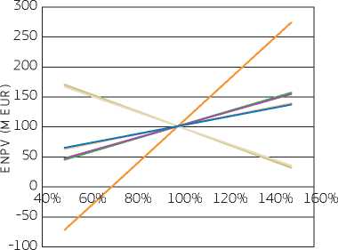
— Econ./Fin. Investment cost
— Econ./Fin. O&M costs (excl. reinvestments)
— Waste flow
— Econ./Fin. Electricity Price
— Econ./Fin. Heat Price
— Shadow price of CO2
— Shadow price of landfill space
Change in variable
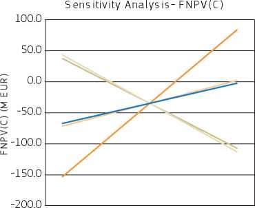
40% 60% 80% 100% 120% 140% 160%
Change in variable
The sensitivity analysis shows that in the economic analysis, only the waste input, and to a lesser extent the investment and operating cost as well as the economic cost of heat and the shadow price of CO2, constitute critical variables. In the financial analysis, on the other hand, most of the tested variables are critical for the FnPV(C)242' This can be explained by the fact that the FNPV(C) is not far from 0 (in which case the project investment would be sufficiently profitable without any external support).
With regards to the waste input, which appears as the most critical variable in both cases, it needs to be noted that the demand analysis was carried out based on conservative assumptions on waste generation both at regional level and in the three large towns that are promoting and co-financing the project. Still, the demand analysis shows that the three towns alone can easily provide the required amount of waste to ensure that the design capacity of the plant is used to the maximum extent over the short, medium and long term. This would still hold true even if source separation of recyclables in the three towns should develop better than expected. Hence, the probability of a decrease of the annual waste throughput equal to the switching value for the ENPV is very low. A higher annual throughput than the designed capacity is not possible, so the switching value for the FNPV(C) is purely theoretical.
With regards to the project costs, unit costs calculated for both construction and operation of the plant compare very well with those of similar projects recently implemented and currently in operation in the EU. The investment cost estimates have also been confirmed in consultations with manufacturers of plants and equipment to cross check with current market conditions. With regards to the disposal costs for waste produced in the WtE plant, it can be said that these were consulted with disposal companies operating in the region. Environmental assessments confirm the legality and viability of the proposed disposal methods. Consequently, there is no reason for serious doubt in the reliability of any of the project's cost estimates, so that the switching values for the investment and O&M cost can be considered as highly unlikely to occur in reality.
With regards to the estimation of the economic benefit of replacing heat production from coal with heat produced by the project, it is to be noted that the value assumed for the avoided cost of heat production has been calculated based on conservative assumptions on the price of coal, as well as on capital and operating cost for heat production. It is therefore quite unlikely that its switching value (required for the ENPV to become 0), which is around -91 %, could somehow materialise. This would not be the case even if the internalised penalty for security of supply of coal were removed or if the long-term marginal cost of heat production were replaced with the short-term marginal cost (as in the financial analysis).
On the assumed financial heat price received for heat supplied, it should be mentioned that the conditions for the heat off-take (including the price) have been negotiated in advance with the local district heating provider, with whom a basic agreement exists that is also supported by the local government of the municipality in question. An important decrease of the heat price below the assumed level appears thus highly unlikely.
With regards to the assumed shadow price of CO2, it has been noted already that the assumed values are estimates used by the EIB, which gives them a high degree of credibility.
With regards to the project facility's gate fee, which is also very critical for the financial analysis, it should be mentioned that the values assumed in the analysis have been discussed and approved by the municipal governments of the three towns participating in the project which is why these are not likely to change in the future.
All in all, the assumptions made for the critical variables of the project appear to be well founded which makes the results of the CBA appear robust.
Based on the results of the sensitivity analysis and taking into account uncertainties related to aspects not directly reflected in the CBA calculations, a risk matrix was prepared in order to identify possible risk prevention and mitigation measures.
|
Risk description |
Proba bility* (P) |
Sever ity (S) |
Risk level* (=P*S) |
Risk prevention/ mitigation measures |
Residual risk after prevention/ mitigation measures |
|
Demand side risks | |||||
|
Available waste flow is much lower than the design capacity of the plant |
B |
III |
Moderate |
Demand analysis is carried out based on conservative assumptions on waste generation in the project’s catchment area which are comparable with assumptions made in other regions in the country. Local governments of the three towns participating in the project control the waste flow within their collection zones and will produce more than sufficient residual waste to ensure maximum use of the demand capacity in the short, medium and long term. Function in charge: project beneficiary in coordination with municipal governments of the three towns participating in the project |
Low |
|
Risk description |
Proba bility* (P) |
Sever ity (S) |
Risk level* (=P*S) |
Risk prevention/ mitigation measures |
Residual risk after prevention/ mitigation measures |
|
Composition and calorific value of the actual input waste are outside of the range used to design the incineration plant |
C |
III |
Moderate |
Changes in composition of household waste and separation rates of recyclables and other waste fractions assumed in the demand forecast are plausible and based on developments observed also in other countries. Calorific value assumed for the input waste is in line with that of waste of other urban areas within the country and abroad. In case of seasonal fluctuations in waste composition, appropriate mixing with waste from different sources from within the same catchment areas is possible. Function in charge: project beneficiary in coordination with municipal governments of the three towns participating in the project |
Low |
|
Uncertainty with regards to off-take of heat produced in the plant |
C |
IV |
High |
Heat off-take agreement has been negotiated with local district heating provider and is reflected in a declaration of intent signed by the two parties. Agreement is supported by the local government of the relevant town. Function in charge: project beneficiary, local government of the relevant town |
Low |
|
Financial risks | |||||
|
Investment cost overrun |
C |
III |
Moderate |
Investment cost estimates compare well with costs experienced with similar projects implemented in the EU in the last years. Consultations with plant and equipment manufacturers were carried out to cross-check estimates with current market conditions. Publication of contract notices in the Official Journal of the EU to ensure wider competition. Function in charge: project beneficiary |
Low |
|
Operating cost overrun |
B |
III |
Moderate |
Operating cost estimates compare well with costs experienced with similar projects in operations. Consultations with plant and equipment manufacturers were also carried out to cross-check estimates. Real increases in staff costs have been considered in the operating cost forecasts. Electricity consumption, which makes up 13 % of total O&M cost is largely covered by own production. Waste disposal costs have been consulted with disposal companies active in the region. Function in charge: project beneficiary |
Low |
|
Problems with availability of local co-financing |
C |
IV |
High |
National public grants confirmed through commitments of the national government to co-finance the relevant OP. Regional Government and involved Municipalities have all provided written commitments to (co-) finance the project, interests during construction and initial working capital. Project beneficiary is seeking a loan from the EIB to co-finance the project, for which first negotiations have started. Function in charge: Ministry of Finance, managing authority responsible for the OP, regional government, municipal governments of the three towns participating in the project, project beneficiary |
Moderate |
|
Risk description |
Proba bility* (P) |
Sever ity (S) |
Risk level* (=P*S) |
Risk prevention/ mitigation measures |
Residual risk after prevention/ mitigation measures |
|
Delays in project preparation and approval leading to late availability of EU grant co-financing |
C |
III |
Moderate |
Involve JASPERS technical assistance early in the project cycle to reduce time for project approval. Function in charge: Managing authority responsible for the OP, project beneficiary |
Low |
|
Shortfall in revenues from gate fees and sales of materials and energy jeopardises debt service |
B |
IV |
Moderate |
Proposed gate fees for the WtE have been agreed in advance with the three towns participating in the project. The heat off-take price has been negotiated and agreed in principle with local DH service provider and is reflected in a declaration of intent signed by the two parties. The agreement includes provisions for regular price adjustments for inflation and for changes in the price of coal or the price paid by the district heating operator for CO2 emissions. The off-take price for electricity is a long-term average which has been assumed in accordance with current forecasts of demand and supply. The scrap metal price is set based on the current market price which is considered a conservative assumption for the future (demand growth is expected to outpace supply so prices are not expected to fall). Function in charge: project beneficiary |
Low |
|
Implementation risks | |||||
|
Problems with land purchase |
A |
II |
Low |
Land is owned by one the municipalities promoting the project. Conditions for land purchase have already been agreed in principle. Function in charge: project beneficiary. |
Low |
|
Problems with public opposition to the project |
D |
IV |
Very high |
The public consultation process required as part of the EIA is well advanced and concerns raised during public hearings do not represent any critical issue for the project. Recommendations made by environmental NGOs have been partially incorporated into the project. Publicity measures aimed at informing the public about the project and its objectives are included in the project. Function in charge: project beneficiary |
Moderate |
|
Delays related to extension of tender procedures |
C |
III |
Moderate |
Promoter’s procurement division to be supported by specialised technical assistance. Appropriate time contingencies are factored into the project schedule. Function in charge: project beneficiary |
Low |
|
Operational risks | |||||
|
Limits for emissions of pollutants to air/ water are exceeded |
A |
II |
Low |
Selection of proven, best-available technologies for flue gas treatment and wastewater treatment facilities Function in charge: project beneficiary. |
Low |
* Evaluation scale: Probability: A. Very Unlikely; B. Unlikely; C. About as likely as not; D. Likely; E. Very Likely.
Severity: I. No effect; II. Minor; III. Moderate; IV. Critical; V. Catastrophic.
Risk level: Low; Moderate; High; Very High
The risk analysis convincingly shows that the residual risks for the project are either low or moderate as a result of the measures already implemented to prevent the occurrence of the identified risks and/or to mitigate their adverse impact in case these should unexpectedly materialise. All in all, the overall level of residual risk is deemed to be fully acceptable, It can be therefore concluded that, provided that the project is awarded with the EU funds as expected and recommended, the probability of the project failing to attain its targeted objective at a reasonable cost is only marginal.
Investments in energy infrastructures in EU Member States are driven by specific challenges affecting the national, regional and international energy markets. The main issues that are specific to the EU are related to security and reliability of supply, and affordable energy prices for consumers. Also, global concerns for climate change call for the need of progressively substituting fossil-based energy fuels with more sustainable sources. Related to this, another important driver is derived from the challenges posed by the growing penetration of power generation from intermittent renewable energy sources, particularly wind and solar, to the entire electrical system, and to the power grid in particular.
The objectives of European energy policy are the construction of appropriate cross-border interconnections, diversification of supply sources and routes, promotion of energy efficiency, and the acceleration of the transformation to low-carbon energy. Their strategic importance is reaffirmed in the overarching Europe 2020 strategy for smart, sustainable and inclusive growth in the EU and in its flagship initiative entitled ‘resource-efficient Europe'. In particular, this flagship aims to help decouple economic growth from the use of resources, support the shift towards a low-carbon economy, increase the use of renewable energy sources, modernise the transport sector, promote energy efficiency, enhance competitiveness and promote greater energy security. Targets have been set by the EU to achieve a 20 % reduction of GHG emissions below the 1990 level, a 20 % share of energy from renewable energy sources and a 20 % reduction in the use of primary energy by the improvement of energy efficiency by 2020. Further targets have been set by the EU for 2030 as part of its policy framework for climate and energy in the period from 2020 to 2030243: a binding EU-wide target to reduce GHG by at least 40 % below the 1990 level, a binding EU-wide target to increase the share of renewable energy to at least 27 %, as well as an indicative target to increase energy savings through the improvement of energy efficiency by 27%. The importance of diversifying oil import sources in order to ensure not only financial savings, due to increased competitiveness, but also energy security, and the need for upgrading Europe's network, including Trans-European Energy Networks, are also stressed in European strategic documents.
Roadmaps, action plans and regulatory documents have been developed by European authorities. EU strategic goals have been translated by Member States into more concrete measures to be implemented in the upcoming years, tailored to the specific national and regional investment priorities.
During the 2014-2020 period, the ERDF and the Cohesion Fund will invest in supporting the shift towards a low-carbon economy in all sectors (thematic objective 4), including investments in energy efficiency, renewable energy244, smart distribution systems and high-efficiency co-generation of heat and power based on useful heat demand. In addition, the ERDF could also invest in improving energy efficiency and security of supply through the development of smart energy distribution, storage and transmissions systems, and through the integration of distributed generation from renewable sources245. In general, investments to achieve the reduction of greenhouse gas emissions from activities falling under Annex I of Directive 2003/87/EC (the Emissions Trading System Directive) cannot be supported by the ERDF or the Cohesion Fund. The rationale for this exclusion is that such investments would just foster a reduction in the price of emission permits, without achieving additional decreases in the volume of emissions (as the number of permits remains fixed, and thus the volume of greenhouse gas emissions).
A selective list of policy and regulatory documents for the energy sector is provided in the box below.
Communication from the Commission, ‘A policy framework for climate and energy in the period from 2020 to 2030’, COM(2014) 15. Green Paper, ‘A 2030 framework for climate and energy policies’, COM(2013) 169 final.
Regulation (EU) No 347/2013 on guidelines for trans-European energy infrastructure and Commission Delegated Regulation (EU) No 1391/2013 amending Regulation (EU) No 347/2013 of the European Parliament and of the Council on guidelines for trans-European energy infrastructure as regards the Union list of projects of common interest.
Regulation (EU) No 1316/2013 establishing the Connecting Europe Facility.
Report from the Commission to the European Parliament and the Council, ‘The state of the European carbon market in 2012’, COM(2012) 652 final.
European Commission Communication ‘Making the internal energy market work’, COM(2012) 663 final.
European Commission Communication ‘Energy Roadmap 2050’, COM(2011)885 final.
European Commission Communication ‘A Roadmap for moving to a competitive low carbon economy in 2050’, COM(2011) 112 final. European Commission Communication ‘Roadmap to a Resource Efficient Europe’, COM(2011) 571 final.
Commission Staff Working Paper ‘Energy infrastructure investment needs and financing requirements’, SEC(2011) 755 final. ENTSO-E - European Network of Transmission System Operators for electricity, ‘Ten-year Network Development Plan’.
ENTSOG - European Network of Transmission System Operators for Gas, ‘Ten-Year Network Development Plan’.
Member States’ National Renewable Energy Action Plans.246 Member States’ National Energy Efficiency Action Plans.247
European Commission Communication, ‘Delivering the internal electricity market and making the most of public intervention’, COM(2013) 7243 final.
European Commission Communication, ‘Renewable Energy: a major player in the European energy market’, COM(2012) 271 final.
European Commission Communication, ‘Smart Grids: from innovation to deployment’, COM(2011) 202 final.
Directive 2009/72/EC concerning common rules for the internal market in electricity and repealing Directive 2003/54/EC and Regulation 714/2009.
Directive 2009/28/EC on the promotion of the use of energy from renewable sources and amending and subsequently repealing Directives 2001/77/EC and 2003/30/EC.
Regulation (EU) No 994/2010 concerning measures to safeguard security of gas supply and repealing Council Directive 2004/67/EC.
Directive 2009/73/EC on common rules for the internal market in natural gas and repealing Directive 2003/55/EC and Regulation 715/2009.
Commission Staff Working Document, Guidance note on Directive 2012/27/EU on Energy Efficiency, amending Directives 2009/125/EC and 2010/30/EC, and repealing Directives 2004/8/EC and 2006/32/EC.
Directive 2012/27/EU on Energy Efficiency.
Directive 2010/31/EU on the Energy Performance of Buildings.
Understanding the context in which the project is implemented is the first step of any project appraisal. This is particularly important for energy projects, as they are usually part of a network that extends at national or international level, thus making the project's sustainability and performance subject to a large number of external factors. The baseline context elements recommended to be described for energy projects are shown in the following table.
Table 5.1: Presentation of the context: Energy sector
|
Information | |
|
Socio-economic-political trend |
- National and regional GDP growth - Income disposal - Demographic change - Energy intensity of the economy250 - Fuel price trends |
|
Geographical factors |
- Weather and climate conditions - Type and quantity of energy sources and fuels available within the national territory (energy balance) - Degree of interconnection and integration with other countries |
|
Political, institutional and regulatory factors |
- Reference to EU directives and sector policy documents (see above) - Reference with the priority axis and the interventions areas of the operational programme (OP) - Reference to the short, medium and long-term national, regional and local planning documents and strategies, including for example the National Renewable Energy Action Plan - Political factors influencing the energy market (such as conflicts or political tensions involving the fuel exporter countries) - Regulatory and controlling authority(ies) and its/their role |
|
Existing service market conditions |
- Structure of the market: energy utilities, wholesalers, retailers, types and number of final consumers - Degree of vertical integration of the market and information about market liberalisation and competition in the sector - Tariff and/or energy price system and consumer price trend |
|
Existing service technical conditions |
- Volumes of energy production, intermediate and final consumption, import and export by type of energy (electricity, natural gas, oil, heat, secondary bio-fuels, etc.) and energy sources/fuels for electricity generation - Import dependency rate - Load profile and load factor of technologies interested in the project - Seasonal and daily trend of energy consumption - Information about historic and current energy production, consumption and trade patterns - Degree of achievement of EU/national targets for the energy sector - Planned and/or recently executed investments that may affect the project performance - Technical characteristics of the service currently provided - Service quality and reliability - Infrastructure production / transportation capacity and energy storage capacity |
Source: Authors
The most direct objective of energy projects is to address one or more of the challenges that affect the energy systems in Europe, which were briefly recalled in the introductory section. In more detail, energy projects generally aim at:
• developing new energy capacity to meet increasing energy demand;
• developing new energy capacity to reduce energy import dependency;
• extending the energy supply network to reach non-served areas; 248
• diversifying energy sources and supply markets;
• integrating the national energy market to other countries better, so as to ensure an alignment of consumer energy prices throughout the EU;
• improving technical reliability and security of energy supply, and avoiding energy interruptions;
• increasing energy efficiency in production facilities by reducing energy losses, modernising existing plants for energy production and promoting co-generation;
• increase the efficiency and quality of the energy system by technically and/or operationally improving the transmission or distribution of energy;
• increasing consumption energy efficiency, e.g. of residential and/or public buildings and/or technical installations, to reduce their overall energy consumption;
• reducing greenhouse gases and pollutant emissions produced by the energy sector by substituting fossil fuels with more sustainable energy sources, such as renewable ones (wind, solar, hydropower, biomass, etc.).
Having defined the objective of the intervention, the next step is to present in detail the proposed project to be implemented. The focus is on the following two categories of projects:
• construction, modernisation and quality improvement of energy production plants, storage, transport, transmission and distribution networks;
• actions to improve the efficiency of energy consumption, i.e. energetic rehabilitation of public and private buildings and industrial production systems.
Information and data about the project's engineering features, technical characteristics, expected effects, and types and numbers of consumers served are to be provided. See the typical categories of investment costs in section 5.5. The implementation of any investment project should be justified against a set of feasible alternative options that allow achieving the same objective (see section 5.6).
The following table provides examples of energy investments, together with the following typologies:
Table 5.2 Examples of energy investments
|
Energy production, storage, transport, transmission and distribution |
Electricity |
- Construction of a power plant that produces electricity from a given renewable or non-renewable source/fuel - Modernisation of an existing power plant to increase energy production capacity and/or energy efficiency and/or substitute the energy fuel/source - Construction/modernisation of a power transmission line within the country or to other countries - Construction/modernisation of the electricity distribution system (electrical substations, dispatch system, electricity transmission grid) - Development of smart transmission and distribution systems (smart grids) - Development and expansion of electricity storage facilities |
|
Natural gas |
- Construction/modernisation of liquefied natural gas (LNG) regasification terminals, underground storage facilities, etc. - Construction of a new or the expansion of an existing transport gas pipeline within the country or linking the national network to the foreign gas supply systems - Modernisation of the already existing gas supply system | |
|
Heat |
- Construction/modernisation of a boiler station or thermal power plant for heat generation or co-generation - Construction/modernisation of a district heat distribution system | |
|
Second-generation biofuels |
- Construction of plants for second-generation biofuels production | |
|
Consumption energy efficiency |
- Refurbishment of public buildings (schools, hospitals, etc.) for improving their energy characteristics - Refurbishment of apartment blocks and other private buildings to improve their energy characteristics - Measures for improving energy saving and efficiency in industrial productive systems251 |
Source: Authors
Both demand and supply of energy in a given market need to be assessed and forecasted for any energy project. This is particularly important for projects involving the production of electricity: due to the limited technological possibilities of storing electricity, a balance between demand and production should always be ensured in order to avoid service disruption. Matching demand and supply forecast is also relevant to gas projects, even if line pack, storage in caverns, aquifers, depleted fields or other facilities (like LNG) are, in principle, possible over long periods of time: actually, the supply of gas from abroad often relies on long-term contracts, so as to stipulate which reliable demand estimates are needed, particularly to ensure service reliability, even during peak demand periods.
Some indications on how energy demand and supply can be forecasted for the purpose of the financial and economic analyses are provided below.
Energy products (natural gas, electricity, heat and biofuels) can be demanded by final consumers, i.e. households, commercial activities and industries or public bodies, and intermediate consumers that transform an energy product into a different one (natural gas can be combusted to produce heat or electricity). When forecasting energy demand of both categories of energy projects (i.e. energy production, transport, transmission and distribution projects, and projects for energy-efficient consumption), different factors need to be taken into account and duly analysed. The most important ones251 are:
• demographic dynamics: the total energy demand is directly related to the size of population;
• economic trend (e.g. gross domestic product, GDP, growth and per capita GDP): a fast-growing economy generally demands a higher quantity of energy than a flat economy; in parallel, higher standards of living are associated with a higher demand for energy;
• weather and climatic conditions: they largely affect the demand for heating and cooling;
• tariff system: it could affect the level of consumption, but also the timing, if discounted prices are provided during off-peak hours;
• particular energy efficiency developments in energy transportation/transmission and/or energy consumption (i.e. through targeted investments): they can also notably affect total gross energy demand.
The most important input data to be considered for forecasting energy demand are:
• annual total and average consumption of energy products, e.g. in TWh/year (for electricity) or bcm/year (for gas), by type of consumers. The following categories of consumers are generally considered:
- household/commercial final consumers,
- industrial final consumers, and
- energy transformation sector;
• the peak demand, generally expressed in GW for electricity and mcm/day for gas;
• variability of seasonal and daily levels of consumption;
• annual export demand.
For energy production, transport, transmission and distribution projects, the project promoter should provide projections related to the level of energy produced and/or transported/transmitted/distributed by the project under assessment. The market shares of key energy producers, wholesalers and retailers should also be analysed and projections of supply of alternative energy products provided. A variation in the supply of alternative energy sources could actually significantly affect the project performance and the energy mix to be considered in the counterfactual scenario (see section 5.8.1).
The main factors affecting the level of energy supply associated with the project are:
• national and international socio-economic and political factors influencing the fuel price dynamics;
• political decisions about the discontinuation of certain types of energy sources and fuels (e.g. nuclear power);
• system of incentives on certain types of energy sources and fuels (e.g. subsides on renewable sources);
• environmental requirements imposing additional costs to energy production;
• structure, territorial size, degree of integration and performance quality of the energy system (both production facilities and the transportation and transmission/distribution networks);
• market structure, particularly related to the number of competitors and the degree of market openness and integration into other markets.
The input data required to determine the present and future levels of energy production and which need to be made explicit in the project appraisal includes:
• structure of the electrical grid or of the transport/distribution networks;
• type of plant and/or technology;
• energy source or fuel used;
• total installed capacity;
• net capacity or utilisation rate of the infrastructure, defined as the ratio between the actual output expected to be supplied and the maximum possible outputs;
• annual volume of imported energy products;
• efficiency, which varies by type of fuel and energy production technology;
• estimated losses of energy produced and/or delivered;
• storage capacity (for natural gas and electricity).
Alternative options of energy projects should be discussed and compared with each other on the basis of the following information:252
• the characteristics of the present and future energy demand and supply (see section 5.5);
• the environmental conditions in the immediate project area, in particular with regards to air pollution;
• available technological alternatives: the same energy can be produced/transported/stored by a variety of technologies, each one with different degrees of efficiency, capacity and environmental impact;
• available sources for electricity production: some areas might not be provided with particular energy sources (e.g. water basins, sufficient solar exposure, etc.);
• possible routes for energy transport, transmission/distribution network;
• possible synergies with the deployment of NGA infrastructures (especially relevant for smart grids);
• applicable regulations limiting technological options (e.g. regulations forbidding energy production from nuclear power);
• notable negative public opinion / strong public opposition to certain technologies in the given project area/country;
• different peak-load arrangements.
Apart from the general costs for planning and design, construction engineering and publicity, investment costs for energy projects typically include:
• land acquisition and purchase of rights of way;
• decommissioning/dismantling/demolition costs borne when rehabilitating old energy-generation facilities;
• technological plant installations and equipment;
• mobile equipment required for operations;
• connections to the relevant utility networks;
• road access;
• skilled and non-skilled labour costs;
• information technologies, particularly relevant in case of smart grid projects;
• mitigation measures for environmental protection253;
• testing and training of operational staff before start of operations.
The investment cost of the project could also be presented per capacity installed (e.g. EUR/KW for electricity generation, EUR/m3 for gas storage capacity) or length of power lines/pipelines (EUR/km), in order to allow for comparisons and benchmarking to similar projects.
Operating and maintenance (O&M) costs of energy projects can be differentiated between variable and fixed costs, depending on whether they vary with the quantity of energy produced/distributed or not. Fixed O&M costs, whose magnitude depends on the type of project, usually include:
• cost for public concessions fees or other permits;
• general overheads;
• insurance costs;
• labour costs;
• periodic fixed maintenance and repairing costs.
The most relevant variable operating costs are:
• energy fuel costs;
• variable overheads;
• utilities;
• other goods and services for energy production or transportation/transmission/distribution;
• waste disposal costs (including solid waste and waste water);
• for projects involving the construction or modernisation of energy production plants, the cost of greenhouse gas (GHG) emission allowances purchased within the European Emission Trading System (ETS)254, or of similar permits and certificates issued by the different national systems for energy projects producing GHG emissions, have also to be considered as part of the project O&M costs, as far as they represent real cash flows255;
• costs for dismantling and decontamination (if relevant) after decommissioning of large facilities at the end of their economic life. These costs should be duly substantiated with references to cost experiences with comparable facilities that were dismantled in the past.
Revenues are generally associated with energy projects for production, transport, transmission and distribution and not to projects
for energy-efficient consumption. The main typologies of revenues related to these can be classified under the following categories:
• energy or fuel sales: a tariff or a unit price, which is paid by consumers of the energy supplied by the project, usually made of a combination between a fixed and a variable component. Both the tariff and the unit price may depend on a large number of factors, such as the level of consumption, the timing of consumption (during peak or off-peak hours) and the type of user. Also, the tariff could include an incentive component (e.g. feed-in tariff), usually aimed at rewarding renewable energy producers with higher energy prices than the energy price applying to other energy producers over the same market;
• transport or other service sales: a tariff or a price, which is paid by users of the project infrastructure for the service of transporting electric energy through a grid, or heat and gas through a pipeline network. Similarly, a price can be paid for other types of network and ancillary services (measurement, supply adjustments, balancing, capacity payments, etc.). Even in this case, the tariff or price, which generally encompass fixed and variable components, depends on several factors: among others, the amount of capacity reserved, energy transported, the type of service, the timing of the required service, the duration of the contract, etc.;
• sale of energy allowances: for those specific types of projects falling under the ETS Directive and which are eligible for the ERDF or Cohesion Fund, if ETS allowances or similar certificates compensating for the reduced production of GHG emissions are sold on the national or European market (and this gives rise to a real cash flow for the project operator), the resulting revenues have to be included among the project inflows.
Energy projects can produce different social benefits and costs, depending on the specific typology of the project implemented as compared with the counterfactual scenario.
Sub-section 5.8.1 provides a presentation of the main effects usually associated with the construction, modernisation and quality improvement of energy supply networks and/or energy production plants and discusses the methodologies recommended for their evaluation.
Sub-section 5.8.2, instead, is focused on the benefits produced by energy efficiency projects for public and private buildings and industrial productive systems.
Various types of projects for energy production, storage or transport/transmission/distribution are generally associated with
benefits, such as:
• increase and diversification of energy supply to meet increasing demand;
• increase of security and reliability of energy supply, i.e. reduction in the frequency of episodes of power or gas interruptions during the daytime or periods of the year or in geographical areas;
• reduction of energy costs for substitution of the energy source, because of the change of the country from which the energy is imported, a substitution of self-production with import or of import with self-production, and the displacement of the source or fuel for electricity production;
• market integration, i.e. the ability of a power system to reduce congestion so that energy markets can trade power in an economically efficient manner and achieve higher socioeconomic welfare;
• improved energy efficiency leading to a reduction in the cost of production, storage or transport/transmission/distribution per unit of energy.
Two environmental externalities are common to all these types of energy projects. These are the variations of GHG emissions
and air pollution (e.g. in particular, airborne pollutants such as SO2, NOx, particulate matter (PM), volatile organic compounds
(VOCs), mercury and other heavy metals, etc.).
Table 5.3 Typical benefits of energy projects
|
Economic benefit |
Type of effect |
Examples of typical projects |
|
Increase and diversification of energy supply to meet increasing demand |
Direct |
Construction of a new energy production plant Increase of production capacity of an energy facility Construction/expansion of energy storage facilities Construction of an interconnector or LNG regasification facilities to expand the volume of imported energy |
|
Increase of security and reliability of energy supply |
Direct |
Construction of a new energy production plant Construction/modernisation of energy supply systems within the country Integration of electricity and natural gas networks into EU electricity and gas supply systems Construction/expansion of energy storage facilities Development of a smart distribution system (smart grids) Integration of renewable energy sources in the power network256 257 |
|
Reduction of energy costs for substitution of the energy source |
Direct |
Construction of a new energy production plant displacing existing ones Construction/modernisation of energy supply systems within the country Development of a smart distribution system (smart grids) |
|
Market integration |
Direct |
Construction/expansion of storage facilities Development of new cross-border transmission lines |
|
Improved energy efficiency |
Direct |
Modernisation of energy facilities to improve production efficiency Modernisation of an energy distribution system to reduce losses |
|
Variation of GHG emissions |
Externality |
All types of energy projects |
|
Variation of air pollutant emissions |
Externality |
All types of energy projects |
Source: Authors
Table 5.4 presents the different methods suggested to evaluate the above-mentioned benefits, along with the counterfactual scenario usually adopted. Methodologies are more extensively discussed in the following sections. The case study on the gas pipeline, at the end of this chapter, presents a worked example for the evaluation of the direct benefits ‘increase of energy supply to meet increasing demand' and ‘reduction of energy costs for the substitution of the energy source'.
Table 5.4 Methods to value the benefits of energy projects
|
Economic benefit |
Valuation method(s) |
Counterfactual |
|
Increase and diversification of energy supply to meet increasing demand |
Willingness to pay (WTP) for increased energy consumption |
- ‘Do-minimum’ option: next best alternative to meet increased demand |
|
Increase of security and reliability of energy supply |
- WTP for increased security and reliability of supply (e.g. value of lost load in electricity) - Avoided social cost for non-served energy |
- Business as usual, or - ‘Do-minimum’ option: next best alternative to increase security and reliability of energy supply |
|
Reduction of energy costs for substitution of the energy source |
Variation in economic costs of the substituted/ substituting energy source/fuel |
- Business as usual: the same energy source or electricity production mix continues to be used |
|
Market integration |
- Cost savings - Increased socioeconomic welfare (consumer surplus + producer surplus + congestion rents for electricity) |
- Business as usual |
|
Improved energy efficiency |
Variation in economic costs of the energy source/fuel |
- Business as usual |
|
Variation of GHG emissions |
Shadow price of GHG emissions |
- Business as usual |
|
Variation of air pollutant emissions |
Shadow price of air pollutants |
- Business as usual |
Source: Authors
The estimates of benefits can be commented on to show the contribution of the project to some of the objectives of the
EU energy policy. In particular:
- if the project concerns the displacement of an imported energy product (e.g. electricity) with self-production at a lower cost, the estimate of reduced energy production/supply costs from the substitution of the energy source captures the decreased energy import dependency of the country;
- if the project allows importing energy at a cheaper price and displacing less efficient national generation, thanks to the increased interconnection capacity of the country, the benefit would reflect the increased integration of the EU market;
- if the project concerns the replacement of a fossil fuel with a renewable energy source, the estimate captures the progress towards a low-carbon economy and the increased diversification of energy sources;
- if the project concerns interventions to reduce energy losses/consumption so as to lower production/consumption costs, the estimate captures an increase of energy efficiency and the reduction of GHG emissions and pollutants.
5.8.1.1 Increase and diversification of energy supply to meet increasing demand
A project aimed at increasing (and diversifying) the current total level of energy production in a country or a region in order to meet growing demand, or at extending the energy network to areas currently not served, yields higher revenues for the energy producer/distributer, which are accounted for in the financial analysis.
While, in the case of power, average wholesale prices do generally reflect the marginal cost of energy generation, the socioeconomic value ascribable to the improved energy service is not properly reflected in observed prices to final users, due to various market distortions, like feed-in tariffs. For this reason, in the economic analysis the financial revenues should be replaced by a shadow price computed as the users' willingness-to-pay for receiving one more unit of energy.
The WTP can be estimated in three possible alternate ways:
• revealed preference method: the avoided costs associated with the alternative systems of energy production (e.g. self-generation of electricity and heat through micro turbines and boilers respectively) that the user would employ in order to meet the demand not addressed by the existing supply system can be considered as a proxy of the economic value of increased energy consumption;
• stated preferences method: an ad hoc contingent valuation can be put in place to derive the maximum price that the project's users would be willing to pay for one more unit of energy consumed;
• benefit transfer: the economic value for one more unit of energy consumption estimated through a contingent valuation for other countries can be plugged into the project's economic analysis, provided that the necessary adjustments are made in order to better adapt the value to the specificities of the project context. In general, the unit economic cost of incremental energy should be adjusted to the national per capita GDP.
Having the WTP for one unit of energy consumed, the benefit can be estimated by multiplying it with the incremental volume of energy consumed.
5.8.1.2 Increase of security and reliability of supply
Some investment projects in the electricity sector - such as the improvement of a power transformer station, the integration of renewable energy sources in the power grid or smart grid projects258 to meet peak demand better - could contribute towards determining a reduction in the frequency of episodes of power disruptions during the day or periods of the year or in geographical areas. Similarly, for projects in the gas sector, such as the construction of liquefied natural gas terminals, the increase of the domestic storage capacity or new pipelines changing or diversifying the source of gas, could help to avoid unexpected gas supply shortfalls. In all these situations, the final energy consumers enjoy the benefit of increased security and reliability of energy supply, which must be properly valued. To this end, two possible approaches could be adopted.
The first one entails the estimation of the users' WTP for increased energy reliability and security of supply. The WTP can be estimated via:
• revealed preferences: if a compensation system for users covering the losses incurred due to a disruption of energy supply is in place, the compensation paid for the quantity of energy not supplied or for the time of disruption can be taken as a proxy of the users' willingness-to-accept for the poor quality of service, which, in principle, should be equal to the willingness-to-pay for an improved service. Alternatively, if there is no compensation system and the project users employ alternative systems of energy production/supply (own systems or provided by others) in order to ensure the continuity of the service even during (usually short) periods of disruption, the total costs associated with these alternative systems can be considered as a proxy of the value of increased reliability of energy consumption. Finally, another method is to consider the avoided cost of ensuring security of supply through the next best alternative (for example, in the case of a gas interconnection project, the next best alternative could be an underground gas storage or a LNG facility);259
• stated preferences: an ad hoc contingent valuation can be put in place to derive the maximum price that the project's users would be willing to pay for a reduction in the frequency/duration of episodes of energy interruptions;
• benefit transfer: the possibility of transferring values of WTP estimated in other countries to the country in which the project is implemented (benefit transfer) should also be examined. However, this method might not be very effective, since the WTP is usually estimated on the basis of customer damage functions (modelling social costs for interrupted energy as a function of the interruption duration), which are very country-specific. Therefore, it is generally recommended to adjust the WTP values to the specificities of the project, otherwise different methods of estimation should be applied.
As a second best option, the project appraiser could value the social cost of non-served energy that is avoided thanks to the project implementation. This cost can be obtained, for example, by dividing the annual gross value added (GVA) by the annual volume of energy (electricity, gas, heat, etc.) consumed in the economy, possibly distinguishing between different economic sectors (e.g. industry, commerce and services, agriculture, fishing, etc.). For domestic consumers, the cost of energy not supplied can be determined in a similar way, by dividing the annual household disposable income by annual domestic energy consumption. This is a very simplistic method, but has the advantage of not relying on direct surveys to assess the consumers' WTP.
The cost of non-served energy should be used to value the additional energy made available in the system thanks to the project, against a without-the-project scenario in which interruptions are more frequent or prolonged. Hence the probability of future energy disruption should be compared to the probability existing without the project implementation, so as to estimate the value of energy of the avoided interruption.
5.8.1.3 Reduction of energy costs for substitution of the energy source
A variety of energy investment projects aims at reducing energy production and distribution costs, by substituting one energy source with another. The concept of energy substitution can be intended in different ways, namely:
• substitution of the energy import country: the project implementation (e.g. a new gas pipeline, a LNG terminal or a high-voltage power line) allows for substituting part (or all) of the energy imports supplied by certain countries with more convenient (i.e. cheaper) energy supplied by a different country;260
• substitution of self-production with import: a project increasing the interconnection of the energy market could allow the substitution of energy produced domestically with cheaper energy imported from another country;
• substitution of import with self-production: the project (e.g. the construction of a new energy generation plant or interventions to increase their capacity) intends to decrease dependency on energy imports by substituting part (or all) of the imports with domestically produced energy;
• substitution of the source or fuel for electricity production; the project allows the production of electrical energy that uses an energy source/fuel in substitution of another one, thus changing the production mix of electricity (e.g. the construction of a new power generation plant for renewable sources to substitute electricity produced from fossil-based sources, or the installation of co-generation plants producing electricity and heat from natural gas instead of oil products).
Of course, these projects could also produce a variation of external costs, such as GHG and pollutants' emissions, and/or a change in energy reliability and security of supply. However, these benefits should be treated as separated (see also the gas pipeline case study and the waste-to-energy case study) and valued as shown elsewhere in this section. The focus here is on the reduction of costs that are possibly experienced by the energy producer and distributer because of the substitution of the energy source.
Note that the project could also be associated with an increase in energy production/distribution costs, for example where projects displace dispatchable fossil-fuel generation with intermittent renewable energy sources, which generally impose an extra cost to the system for balancing (cost of countertrading by the transmission system operator to avoid the overloading of saturated transmission lines or to increase generation when RES production is lower than forecast). An increase of costs imputable to the substitution of energy sources must be valued through the same methodology as presented in this section. However, projects of this type could still produce a net benefit to society if these costs are overcome by other benefits.
In the economic analysis, the variation of the costs related to tradable energy sources (e.g. natural gas and electricity) should be estimated by computing the opportunity cost of the different energy items produced in the project reference markets and the counterfactual scenario.
For projects involving the substitution of the energy source/fuel for electricity generation, the opportunity cost of the substituted and substituting sources/fuels (oil, natural gas, biomass, nuclear, solar, wind, hydro, etc.) should be considered as valuing the variation of energy costs. In general, the most costly source is displaced by cheaper ones, but there may be other power dispatch rules. For this reason, the project promoter is recommended to explain and justify which particular energy source/fuel is identified as the one displaced by the project.
As regards projects for which it is not possible to identify what specific electricity source/fuel will be displaced by the increased project's power production261, a shortcut method for the benefit evaluation is to assess the variation of the energy opportunity cost against a counterfactual one in which the average electricity production mix of the market is taken into account. Hence, the opportunity cost of the substituted electricity would depend on the specific mix of sources/fuels used to produce it: the average of opportunity costs of each source/fuel weighted by the share of electricity produced by each source over the total production should be computed.
The opportunity cost of energy products and sources/fuels should be based on the long run marginal cost (LRMC) of production, reflecting the total social cost incurred to produce an extra unit of energy,262 plus the transport cost of the energy source from the place where it is produced to where it is used, if applicable.
5.8.1.4 Market integration
This benefit is related to price alignment effects across places (for transmission) or time (for storage) thanks to the capacity of exploiting differences in energy prices (e.g. for storage, base vs. peak loads for electricity, summer vs. winter for gas). Market integration in particular reflects the potential benefits of (cross-border) electricity transmission263 or energy storage investments264.
For example, a new cross-border electricity transmission project that increases grid transfer capabilities265 between two bidding countries/areas allows generators in the lower-priced country/area to export power to the higher-priced (import) area, thus reducing the total cost of the electricity supply. This market effect turns into an economic effect when the project contributes to:
• reducing network bottlenecks that restrict the access of generation to the full European market;
• providing a direct system connection to new, relatively low-cost, generation; or
• facilitating increased competition between generators, reducing the price of electricity to final consumers.
The benefit can be estimated as the reduction in generation costs associated with the grid transfer capability variation created by the project.
In the gas sector, storage facilities allow more gas to be bought in summer, when it is readily available and generally cheaper, and withdrawn in winter, when gas may be in short supply and additional volumes will generally be very expensive. In this way no investments are needed to meet increased demand during the winter period. The benefit is given by the difference between the value of summer and winter gas, i.e. by the so-called ‘value of swing'. In practice, the value of swing seen as a difference in the average prices of gas between two different periods shall be multiplied by the working volumes of the gas storage facility along each year of the time horizon of the analysis.
5.8.1.5 Improved efficiency
An improvement of the quality of the energy system can bring increased energy efficiency thanks to a reduction of energy losses or a general improvement of the energy production or transport/transmission/distribution technology, which allows lowering the unit cost of energy. The benefit is enjoyed by the energy producer or distributor, and it could also eventually affect consumer prices. The increase in energy efficiency is valued via the decrease of energy cost, incurred by the energy producer/distributor to produce/distribute the same quantity of energy without the project. Different to the financial analysis, the variation in costs is expressed in terms of the opportunity cost (shadow price) of the energy fuel or source, instead of its actual market price.
The opportunity cost of the energy inputs pertinent to the specific project case reflects the loss to society by the diversion of them from the best alternative use. It should be calculated, as usual, as the long run marginal cost of production and transportation.
Note that the variation in the economic cost of the energy fuel/source due to increased efficiency does not incorporate the full value of external costs (e.g. GHG emissions and pollution), which must be separately assessed (see section below).
5.8.1.6 Variation of GHG and air pollutant emissions
The different stages of the life cycle of energy production plants, from their construction to their operation and eventual dismantling, provoke the emission of greenhouse gases (GHGs), such as, mainly, carbon dioxide (CO2), and, to a lesser extent, also methane and nitrous oxide (CH4 and N2O). In principle, the Emissions Trading System (eTs) or other similar national systems rewarding energy operators that produce low levels of GHGs and penalising those producing high GHGs are conceived to internalise in the project's account the climate change impact. The permit price ideally reflects the loss of profits of the business whose production is crowded-out, i.e. the compensation (permit price) just covers that loss of producer surplus. If so, the permit price reflects a real opportunity cost. According to this perspective, the cost sustained or saved to buy emissions permits should already capture the cost or benefit of the project on climate change.
However, more frequently, the price of allowances cannot be regarded as a reliable economic cost of emissions since it is likely to be distorted, even to high extent, by various country-specific political factors. Therefore, the recommended method for the evaluation of changes in GHG emissions is that of replacing the permit price with unit economic costs.266
Other pollutant compounds are also produced by energy infrastructures, such as sulphur dioxide, nitrogen oxides, non-methane volatile organic compounds as precursors of ozone, particulate matter, mercury and other heavy metals, etc. Even if modern plants are equipped with scrubbers, filters and combustion control equipment that limit the release of these unhealthy pollutants within legally specified levels defined under EU law, a residual is usually still emitted. This represents an external cost that must be valued in the economic analysis. The same approach suggested for the valuation of GHGs applies to pollutants.
The data needed to evaluate the economic costs of GHG emissions and pollution is given below in more detail.
• Changes in GHG emissions and pollutants. All types of power plants produce some GHGs and pollutants during their life cycle (construction, operation, dismantling and fuel), including those fed with renewable energy sources. Therefore, the amount of GHG emissions and pollutants produced by both the project and the counterfactual case have to be quantified, in order to determine the increase or decrease in emissions/pollutants' volume. These have to be consistent with the information provided in the Environmental Impact Assessment Report, whenever required. If the volume of emissions associated with the energy project under assessment is not available, relevant sectorial literature or previous studies can provide benchmark values on emission factors. For example, the CASES database267 contains the default volume of emissions released by different types of electricity and heat generation plants and technologies. Also, the EMEP/EEA air pollutant emission inventory guidebook 2013 provides detailed literature on air pollutant for sectors including energy.
• Unit economic costs. A monetary value reflecting the climate change or pollution cost of different typologies of energy infrastructures must be attributed to the incremental volume of pollutants produced by the project against the counterfactual value. A key reference study providing the unit values of air pollutants produced by energy infrastructures in EU Member States is Extern-E268 through its integrated environmental impact assessment model. Another key reference is the NEEDS Integrated Project,269 which provides unit damage costs for air pollutants from emerging electricity generation technologies. As for climate change, it is suggested to use the values for the shadow price of CO2 as illustrated in section 2.9.9.
Projects involving a refurbishment of public and private buildings or works to improve the industrial productive systems are associated with an increase of energy efficiency, either of the building or of the production system, which is reflected in a reduction of energy consumption costs. Additionally, insulation works and the improvement of heating systems in buildings could determine an increase in the level of inner temperature and, thus, of comfort.
As with any other energy project, the projects aimed at improving consumption energy efficiency are also characterised by environmental externalities, such as variations of GHG emissions and pollution (e.g. in particular, airborne pollutants such as SO2, NOx, PM, VOC, mercury and other heavy metals, etc.).
Table 5.5 illustrates the types of benefits discussed in this subsection.
Table 5.5 Typical benefits of energy-efficient consumption projects
|
Economic benefit |
Type of effect |
Examples of project |
|
Increase of consumption efficiency |
Direct |
Refurbishment of public buildings Refurbishment of flats and private buildings to improve their energy characteristics Measures for energy saving and efficiency improvement of productive systems |
|
Increase of comfort |
Direct |
Refurbishment of public buildings Refurbishment of flats and private buildings to improve their energy characteristics |
|
Reduction of GHG emissions |
Externality |
All types of energy projects |
|
Reduction of air pollutant emissions |
Externality |
All types of energy projects |
Source: Authors
In the next sections, the methodologies used to assess the above-mentioned benefits are presented. For the sake of clarity, Table 5.6 provides a synthetic overview of the evaluation methodologies, including the counterfactual scenario to be assumed in order to evaluate incremental benefits.
Table 5.6 Methods to value the benefits of energy-efficient consumption projects
|
Economic benefit |
Valuation method |
Counterfactual |
|
Increase of efficiency for consumption |
Variation in economic costs of the energy source/fuel |
- Business as usual |
|
Increase of comfort |
Variation in economic costs of the energy source/fuel |
- Economic energy cost sustained to maintain a ‘thermal comfort’ temperature through the without-the-project technology/system of energy production |
|
Reduction of GHG emissions |
Shadow price of GHG emissions |
- Business as usual |
|
Reduction of air pollutant emissions |
Shadow price of air pollutants |
- Business as usual |
Source: Authors
5.8.2.1 Increase of efficiency for consumption
Refurbishment investment projects to improve the energy performance of both public or private buildings (both domestic and business facilities) generally involve insulation works to facades and roofs, the renewal of windows and an improvement to heating systems, and the installation of own-energy generation appliances from renewable energy sources The typical effect that these projects produce is an increase in energy efficiency for consumption. Projects aimed at improving the energy characteristics of productive systems are also expected to generate an increase in energy efficiency. Unlike the energy-efficiency improvement to infrastructures for energy production or transport/transmission/distribution, the benefit here occurs on the energy consumption side; yet the methodology to estimate such a benefit is the same.
The benefit is valued via the decrease of energy cost incurred when attaining the same final useful effect as in the without-the-project scenario. The cost reduction should not be expressed at market prices, but by considering the opportunity cost of the avoided energy input i.e. the fuel saved due to the increased efficiency of the building's heating system or the industry's energy management system in gas or electricity or oil products. Their respective conversion factor should then apply to the project's specific energy input; the saved costs compared to the counterfactual scenario would represent the project's benefit.
5.8.2.2 Increase of comfort
In some cases, besides the reduction of unit costs of energy consumption, interventions aimed at improving the energy characteristics of buildings could also determine an increase of comfort for users, caused by the higher temperature reached inside buildings. Higher temperatures can be reached because, due to the reduction of unit energy costs, consumers decide to increase the temperature level in the premises.
If this additional comfort benefit is expected, the methodology presented in the previous paragraph, focusing on valuing the reduction of unit cost of energy consumption, should be revised and the method presented here should be applied. In other words, when both an increase of comfort and a reduction of energy unit costs are expected, these benefits have to be valued together.
The suggested approach consists of evaluating the savings of energy consumption costs (expressed as the opportunity cost of energy) achieved by the project against a counterfactual case, in which the energy consumption is assumed to be such that the ‘standard' comfort temperature is ensured in the building. Hence, the only difference compared with the method to value the reduction of unit energy costs concerns the selection of the counterfactual scenario.
Alternatively, the benefit can be captured by the expected increase in property values (hedonic price method). In such cases, however, care should be taken to avoid any double counting. The increase of sales and rental prices of properties already includes any cost savings from improved energy efficiency and, in some cases, other aspects such as renewed facades, etc.
The perceived thermal comfort in buildings is country-specific and indications about the minimum or average temperature in public and private buildings for ensuring adequate thermal comfort should be provided by national official documents and guidelines. In general, the standards for warmth are higher than the minimum temperatures recommended by the World Health Organisation, which are 18 °C for healthy people and 20 °C for the sick, disabled, very old or very young.
Some practical examples illustrating how increased energy efficiency in buildings should be valued, in case the projects allow for either a reduction of unit energy cost only or a reduction of unit costs and an increase of temperature, are presented in the box in the next section.
5.8.2.3 Reduction of GHGs and pollutant emissions
Projects in the sector of buildings' energy efficiency could also bring external benefits, such as a reduction of GHGs and pollutant emissions, due to the renovation works reducing heat dispersion and the amount of energy consumption. The economic value of a change in emission of CO2, or other external environmental costs, such as SO2, NO2 and particulate matter, have to be estimated following the same methodology described for the external cost of energy production or transport/transmission/distribution projects.
This case regards a project involving insulation works and the replacement of the heating system, which allows reduced energy-consumption costs to keep the temperature inside the building at the same level as in the without-the-project scenario. It is assumed that an energy bill of 1,000 is annually paid by the owner of the non-renovated building, which corresponds to a temperature of 18 °C. After the project’s implementation, the energy efficiency of the building increases and this is reflected in a decrease of annual energy costs (to 900) that is required to maintain the same inner temperature. The financial analysis records a decrease in operating cost amounting to 100. In the economic analysis, the opportunity cost of energy should be considered, by applying a conversion factor to the cost saving. This is assumed to be here 1.1 (because emission costs are internalised). Thus, the project’s benefit would amount to:
Benefit = (1,000*1.1) -(900*1.1)= 110
This value expresses the benefit of saving energy fuel, valued at its opportunity cost, without affecting comfort. Positive results would also be obtained at temperatures other than 18 °C, whenever a reduction of energy cost is recorded to keep the temperature constant.
Taking the same without-the-project scenario as in case 1, i.e. a temperature before the renovation works of 18 °C, it is now assumed that the project leads to an increase of the inner temperature to the thermal comfort level, assumed to be 22 °C, and at the same time a decrease of energy costs, from 1,000 to 900. The financial analysis would report a saving of 100 at market prices. The economic analysis, instead, should capture both the benefit of the cost saving and the increase of comfort associated with an increase of temperature. To this purpose, it is estimated that, under the counterfactual without-the-project scenario, the thermal comfort of 22 °C would be reached only by raising the energy costs to 1,200. Then the benefit would be as follows:
Benefit = (1,200*1.1) -(900*1.1)= 330
|
Actual temperature without the project |
Actual temperature with the project |
Annual energy cost without the project |
Annual energy cost with the project |
Energy cost savings at market prices |
Economic benefit a shadow prices | |
|
Case 1 |
1—* 00 o n |
1—* 00 o n |
1,000 |
900 |
100 |
110 |
|
Case 2 |
i—* 00 o n |
22 °C |
1,200 |
900 |
300 |
330 |
In the sensitivity analysis, CBA results should be tested for changes in the following variables (where relevant for the project):
• incremental energy demand;
• number of years necessary for the realisation of the infrastructure;
• investment costs (as disaggregated as possible);
• operation costs (as disaggregated as possible);
• maintenance costs;
• market price or opportunity cost of energy sources and products (either for the financial or the economic analysis);
• energy mix displaced by the project;
• energy saved by the project;
• estimated willingness-to-pay for energy consumption;
• estimated willingness-to-pay for increased energy reliability of security of supply;
• gross value added, if used to estimate the cost of non-served energy;
• assumed economic value and/or quantities of GHG emissions and pollutants produced;
• value of life considered for the valuation of the risk of accidents.
Via the sensitivity analysis, critical variables can be identified. On this basis, a fully-fledged (or at least qualitative) risk assessment must be carried out, typically by assessing the risks presented in the following table.
Table 5.7 Typical risks in energy projects
|
Stage |
Risk |
|
Regulatory |
- Changes of environmental requirements - Changes of economic instruments (e.g. renewable energy source support schemes, EU ETS design) - Changes in energy policy (e.g. concerning the discontinuation of certain types of energy sources and fuels) |
|
Demand |
- Demand shortfalls - Unexpected evolution of prices of different competing fuels - Inadequate analysis of climatic conditions affecting the energy demand for heating and/or cooling |
|
Design |
- Inadequate site surveys and investigation - Inadequate design cost estimates - Innovation in energy production/transmission or energy storage technology making the one in the project obsolete |
|
Administrative |
- Building or other permits - Utility approvals |
|
Land acquisition |
- Land costs higher than predicted - Higher costs for the acquisition of rights of way - Procedural delays |
|
Procurement |
- Procedural delays |
|
Construction |
- Project cost overruns - Delays due to unexpected technical difficulties (such as the installation of undersea pipelines or underground power cables) - Delays in complementary works outside the project promoter’s control (e.g. cross-border projects) - Flooding, landslides, etc. - Accidents |
|
Operation |
- Maintenance and repair costs that are higher than predicted - Accumulation of technical breakdowns - Long out-of-service time for accident or external causes (earthquake, flood, sabotage, etc.) |
|
Financial |
- Changes in the tariff system - Changes in the system of incentives - Inadequate estimate of energy price trends |
Source: Adapted from Annex III to the Implementing Regulation on application form and CBA methodology.
The project consists of the construction of a new gas-transmission pipeline between the two gas nodes of Alpha and Beta. The designed maximum transmission capacity is 700,000 m3/h, or 16.8 million m3/day. The investment includes the following main components:
• a 175 km-long steel pipeline with a diameter of 700 mm (DN 700), to be operated at a pressure of 8.4 MPa;
• two intermediate pressure-reduction and metering stations located in Lambda and Theta;
• the installation of fibre-optic communication system.
The project promoter is the national transmission system operator (TSO).
An existing DN 500 pipeline currently transmits gas between Alpha and Beta. The pipeline was built 30 years ago and is operated at full capacity. Following the increase in demand for gas transmission services in the country and the ongoing expansion of the regional underground gas storage (UGS) facilities, the existing pipeline is no longer able to meet incremental demand and ensure reliable supplies throughout the year.270
The project objectives are well aligned with the main goals of priority axis X: ‘Sustainable, secure and competitive energy' of the Operational Programme ‘Infrastructure'. In particular, the investment will contribute to the following OP indicators.
|
Indicator |
OP 2023 target |
Project (% of OP target) |
|
Length of new gas transmission pipelines (km) |
500 |
175 (35 %) |
|
Additional gas transmission capacity (Mm3/day) |
40 |
16.8 (42 %) |
The construction of the new Alpha-Beta gas pipeline will allow the transmission of additional volumes of gas to/from the expanded UGS facilities in Gamma and Delta, as well as from a new entry point to the network, the liquefied natural gas (LNG) terminal currently under construction in Epsilon. Therefore, energy security will be improved by ensuring the continuity of gas supplies during both peak and off-peak periods to the distribution network and to the large industrial customers directly connected to the transmission network.
Also, the increased penetration of natural gas in the country should in the medium to longer term contribute to the replacement of coal and oil products as energy sources. As gas is a relatively clean fossil fuel, the project will indirectly bring about a reduction in emissions of greenhouse gases (GHG) and airborne pollutants, thereby contributing to the sustainable growth dimension of the Europe 2020 strategy.
Natural gas is the third most important source of energy in the country, after coal and oil, accounting for approximately 20 % of total primary energy supply. The total consumption of natural gas was 18 billion m3 in 2013, with peak demand in the transmission system reaching 83 million m3/day on 6 February.
According to the scenarios and forecasts presented in the ‘National Energy Strategy to 2030', the demand for gas transmission across the country is expected to develop as shown in the table below.
|
National gas demand |
2015 |
2020 |
2025 |
2030 |
|
Annual consumption (Gm3/y) |
19.3 |
25.2 |
26.5 |
27.8 |
|
Peak demand (Mm3/day) |
92 |
120 |
126 |
132 |
As regards demand in the project area, an ‘open season' procedure was launched to test the market interest in additional transmission capacity. Compared to a counterfactual scenario without the project - where supply is constrained at the maximum capacity of the existing DN 500 pipeline, the promoter forecasts that the following additional gas volumes are expected to be transmitted as a result of the construction of the new Alpha-Beta pipeline.
|
Demand - project area Incremental gas flows |
2017* |
2020 |
2025 |
2030 |
2035 onwards |
|
Mm3/year |
332 |
348 |
374 |
401 |
428 |
|
PJ/year (at 39.50 MJ/m3) |
13.1 |
13.7 |
14.8 |
15.8 |
16.9 |
* Planned first year of operation
According to the promoter's analysis of the regional gas market, 50 % of the incremental gas supplies associated with the project will be delivered to industrial customers, 35 % to the power sector and the remaining 15 % to the residential/ commercial sector throughout the regional gas distribution system. Although the market shares may to some extent vary over the project time horizon, it was assumed for simplicity in the economic analysis that they remain fixed.
The option analysis prepared in the Feasibility Study assesses the following two sets of options:
• Choice of pipeline alignment. Three different alternative alignments were considered. The project option is selected based on a least cost-path analysis coupled with qualitative analysis of environmental and technical dimensions. The selected pipeline alignment between Alpha and Beta has the following characteristics:
- the lowest ‘levelised unit transmission cost'271, with a value of EUR 7.40/1,000 m3,
- the least interference with natural areas, including Natura 2000,
- it allows the project to be implemented in stages.
• Technical specifications of the pipeline. Further technical analyses were performed to optimise the selection of the pipeline diameter, material and wall thickness. According to the simulations performed by the TSO, a 700 mm diameter is the most efficient solution for the target capacity of 700,000 m3/h, with L485MB steel pipes and a wall thickness of 17.5 mm.
A breakdown of the investment cost, in constant prices, for the selected project alternative is presented in the following table.
|
Project investment cost (millions of EUR) |
Total cost |
Ineligible cost |
Eligible cost |
|
Planning/design fees |
4.5 |
4.2 |
0.3 |
|
7.6 |
6.6 |
1.0 | |
|
Building and construction |
62.2 |
- |
62.2 |
|
Plant and machinery or equipment |
63.5 |
- |
63.5 |
|
Contingencies274 |
- |
- |
- |
|
Price adjustment (if applicable) |
- |
- |
- |
|
Publicity |
0.1 |
- |
0.1 |
|
Supervision during construction implementation |
2.5 |
- |
2.5 |
|
Technical assistance |
0.4 |
- |
0.4 |
|
Sub-TOTAL |
140.8 |
10.8 |
130.0 |
|
(VAT) |
31.0 |
31.0 |
- |
|
TOTAL |
171.8 |
41.8 |
130.0 |
In addition to the costs above, the promoter will have to fund EUR 2.6 million of interest during construction (IDC). Not all costs are eligible for EU support, as some expenditure was already incurred before the beginning of the programming period. The eligible cost amounts to EUR 130 million.
The unit investment cost of around EUR 210/km/cm2 is in line with that of other similar projects recently completed by the promoter in the context of its current Network Development Plan.274
Operating and maintenance (O&M) costs are budgeted at around 2 % of project assets, based on the promoter's cost data on other similar sections of the transmission network. O&M costs include expenses related to gas compression and gas losses, repair and maintenance, insurance and overheads. No asset replacement costs are forecast over the 25-year reference period.
The natural gas transmission activity is regulated by the National Energy Authority so as to allow the TSO to recover the justified costs and earn a return on the Regulatory Asset Base (RAB) based on the contracted transmission capacity and the expected transmitted volumes. Transmission charging in the country is based on an ‘entry-exit' system: tariffs are paid at entry and exit points to/from the transmission system and are independent of location and distance. The gas transmission tariffs consist of two main elements: a fixed ‘capacity fee', in EUR/m3/h, and a variable ‘commodity fee', in EUR/m3. The capacity fee varies depending on the service supplied (e.g. firm vs. interruptible capacity, annual vs. short-term capacity).
As regards the project incremental revenue, this is, for simplicity, calculated in the financial analysis based on the average transmission charge of EUR 25/1,000 m3, multiplied by the incremental gas flows associated with the investment (as identified in the demand analysis). According to the estimates of the TSO, thanks to the EU grant, the tariffs for gas transmission will not have to be increased in real terms, given that the share of project assets co-financed by the EU contribution is excluded from the RAB on which the return-on-capital component of the transmission tariffs is calculated.
The analysis is performed using a 25-year reference period, including three years of investment phase and 22 years of operations. As the average economic life of the project assets is assumed to be 25 years, a residual value is considered in the last year of the time horizon, equal to the discounted value of the net cash flows in the remaining years of life.275 The financial and economic analyses are carried out in constant prices. A 4 % discount rate in real terms is used in the financial calculations, while a 5 % social discount rate is used in the economic analysis, in line with the EU-wide benchmark set by the European Commission.
The project is subject to the rules on State aid and was therefore notified to the European Commission (Directorate-General for Competition) and subsequently authorised. To ensure proportionality of the aid, it was decided that the EU grant would be determined based on the project's ‘funding gap', in line with the applicable Guidelines on State aid for environmental protection and energy276 277.
Based on the costs and revenue assumptions described in the section above, the estimated ‘funding gap rate' is 30 % (discounted net revenue = EUR 90.9 million, discounted investment cost = EUR 129.8 million, see calculation further below). The EU contribution for the project is in this case fixed at EUR 33.2 million, by multiplying the eligible cost shown in section V above (EUR 130 million) by the ‘funding gap rate' (30 %) and by the co-financing rate of the relevant priority axis of the OP (85 %). The remainder of the investment is funded by the promoter with an own contribution and debt, as shown in the following table.
|
Financing Sources |
millions of EUR |
% share |
|
EU grant |
33.2 |
23.1 % |
|
Promoter’s contribution (including financing of IDC) |
60.2 |
42.0 % |
|
Loan |
50.0 |
34.9 % |
|
Total funding278 |
143.4 |
100.0 % |
The loan has a maturity of 15 years. Based on the loan pricing conditions and inflation expectations, an average interest rate of 3 % in real terms is used in the financial analysis to estimate the loan cash flows. The loan is to be disbursed in the first two years of the investment phase. The principal repayment would start in the first year of operation, while a total of EUR 2.6 million of interest charges is paid during construction.
The following profitability indicators (before-tax, real) are calculated - see cash flow tables below:
• Return on investment (before EU grant): FNPV(C) = EUR -39.0 million
FRR(C) = 1.2 %
• Return on national capital (after EU grant): FNPV(K) = EUR -4.2 million
FRR(K) = 3.5 %
The project is expected to be financially sustainable, as cumulative net cash flows are never negative over the project reference period.
|
EU GRANT |
12 3 |
4 5 6 7 8 9 10 11 12 13 14 15 20 25 | |||||||||||||||||
|
Construction |
Operation | ||||||||||||||||||
|
Calculation of the Discounted Investment Cost (DIC) |
NPV 4 % | ||||||||||||||||||
|
Investment cost |
mEUR |
129.8 |
33.2 |
63.6 |
44.0 |
0.0 |
0.0 |
0.0 |
0.0 |
0.0 |
0.0 |
0.0 |
0.0 |
0.0 |
0.0 |
0.0 |
0.0 |
0.0 |
0.0 |
|
DIC / Investment cost cash-flow |
mEUR |
129.8 |
33.2 |
63.6 |
44.0 |
0.0 |
0.0 |
0.0 |
0.0 |
0.0 |
0.0 |
0.0 |
0.0 |
0.0 |
0.0 |
0.0 |
0.0 |
0.0 |
0.0 |
|
Calculation of the Discounted Net Revenue (DNR) |
NPV 4 % | ||||||||||||||||||
|
Incremental gas flows |
Mm3 |
4,861.8 |
0.0 |
0.0 |
0.0 |
332.0 |
337.0 |
342.0 |
348.0 |
353.0 |
358.0 |
364.0 |
369.0 |
374.0 |
380.0 |
385.0 |
390.0 |
417.0 |
428.0 |
|
Average transmission tariff |
EUR/th.m3 |
321.2 |
0.0 |
0.0 |
0.0 |
25.0 |
25.0 |
25.0 |
25.0 |
25.0 |
25.0 |
25.0 |
25.0 |
25.0 |
25.0 |
25.0 |
25.0 |
25.0 |
25.0 |
|
Revenue |
mEUR |
121.5 |
0.0 |
0.0 |
0.0 |
8.3 |
8.4 |
8.6 |
8.7 |
8.8 |
9.0 |
9.1 |
9.2 |
9.4 |
9.5 |
9.6 |
9.8 |
10.4 |
10.7 |
|
O&M cost |
mEUR |
-38.5 |
0.0 |
0.0 |
0.0 |
-3.0 |
-3.0 |
-3.0 |
-3.0 |
-3.0 |
-3.0 |
-3.0 |
-3.0 |
-3.0 |
-3.0 |
-3.0 |
-3.0 |
-3.0 |
-3.0 |
|
Residual value of investments |
mEUR |
7.9 |
0.0 |
0.0 |
0.0 |
0.0 |
0.0 |
0.0 |
0.0 |
0.0 |
0.0 |
0.0 |
0.0 |
0.0 |
0.0 |
0.0 |
0.0 |
0.0 |
21.0 |
|
DNR / Net revenue cash-flow |
mEUR |
90.9 |
0.0 |
0.0 |
0.0 |
5.3 |
5.4 |
5.6 |
5.7 |
5.8 |
6.0 |
6.1 |
6.2 |
6.4 |
6.5 |
6.6 |
6.8 |
7.4 |
28.7 |
|
ELIGIBLE COST (EC) |
mEUR |
130.0 |
|
FUNDING GAP RATE (FGR = (DIC - DNR) / DIC) |
30.0% | |
|
CO-FINANCING RATE OF PRIORITY AXIS (CF) |
85.0% | |
|
EU GRANT ( = EC x FGR x CF) |
mEUR |
33.2 |
|
1 2 3 |
4 5 6 7 8 9 10 11 12 13 14 15 20 25 |
|
Construction |
Operation |
|
Calculation of the Return on Investment |
NPV 4 % | ||||||||||||||||||
|
Investment cost |
mEUR |
-129.8 |
-33.2 |
-63.6 |
-44.0 |
0.0 |
0.0 |
0.0 |
0.0 |
0.0 |
0.0 |
0.0 |
0.0 |
0.0 |
0.0 |
0.0 |
0.0 |
0.0 |
0.0 |
|
O&M cost |
mEUR |
-38.5 |
0.0 |
0.0 |
0.0 |
-3.0 |
-3.0 |
-3.0 |
-3.0 |
-3.0 |
-3.0 |
-3.0 |
-3.0 |
-3.0 |
-3.0 |
-3.0 |
-3.0 |
-3.0 |
-3.0 |
|
Revenue |
mEUR |
121.5 |
0.0 |
0.0 |
0.0 |
8.3 |
8.4 |
8.6 |
8.7 |
8.8 |
9.0 |
9.1 |
9.2 |
9.4 |
9.5 |
9.6 |
9.8 |
10.4 |
10.7 |
|
Residual value of investments |
mEUR |
7.9 |
0.0 |
0.0 |
0.0 |
0.0 |
0.0 |
0.0 |
0.0 |
0.0 |
0.0 |
0.0 |
0.0 |
0.0 |
0.0 |
0.0 |
0.0 |
0.0 |
21.0 |
|
FNPV(C) - before EU grant / Net cash-flow |
mEUR |
-39.0 |
-33.2 |
-63.6 |
-44.0 |
5.3 |
5.4 |
5.6 |
5.7 |
5.8 |
6.0 |
6.1 |
6.2 |
6.4 |
6.5 |
6.6 |
6.8 |
7.4 |
28.7 |
FRR(C) - before EU grant 1.2%
|
1 2 3 |
4 5 6 7 8 9 10 11 12 13 14 15 20 25 |
|
Construction |
Operation |
National Financing Sources
|
Promoter's contribution (including financing of IDC) |
mEUR |
|
Loan |
mEUR |
|
0.0 |
25.1 |
35.1 |
0.0 |
0.0 |
0.0 |
0.0 |
0.0 |
0.0 |
0.0 |
0.0 |
0.0 |
0.0 |
0.0 |
0.0 |
0.0 |
0.0 |
|
25.4 |
24.6 |
0.0 |
0.0 |
0.0 |
0.0 |
0.0 |
0.0 |
0.0 |
0.0 |
0.0 |
0.0 |
0.0 |
0.0 |
0.0 |
0.0 |
0.0 |
Loan Balance
|
Beginning balance |
mEUR |
|
Loan disbursements |
mEUR |
|
Interest payments |
mEUR |
|
Principal repayments |
mEUR |
|
Ending balance |
mEUR |
|
0.0 |
25.4 |
50.0 |
50.0 |
47.3 |
44.5 |
41.6 |
38.7 |
35.7 |
32.6 |
29.4 |
26.1 |
22.7 |
19.2 |
15.6 |
0.0 |
0.0 |
|
25.4 |
24.6 |
0.0 |
0.0 |
0.0 |
0.0 |
0.0 |
0.0 |
0.0 |
0.0 |
0.0 |
0.0 |
0.0 |
0.0 |
0.0 |
0.0 |
0.0 |
|
0.0 |
1.1 |
1.5 |
1.4 |
1.3 |
1.2 |
1.2 |
1.1 |
1.0 |
0.9 |
0.8 |
0.7 |
0.6 |
0.5 |
0.4 |
0.0 |
0.0 |
|
0.0 |
0.0 |
0.0 |
2.7 |
2.8 |
2.9 |
2.9 |
3.0 |
3.1 |
3.2 |
3.3 |
3.4 |
3.5 |
3.6 |
3.7 |
0.0 |
0.0 |
|
25.4 |
50.0 |
50.0 |
47.3 |
44.5 |
41.6 |
38.7 |
35.7 |
32.6 |
29.4 |
26.1 |
22.7 |
19.2 |
15.6 |
11.9 |
0.0 |
0.0 |
|
Calculation of the Return on National Capital |
NPV 4 % | ||||||||||||||||||
|
Promoter's contribution (net of IDC) |
mEUR |
-52.1 |
0.0 |
-24.0 |
-33.6 |
0.0 |
0.0 |
0.0 |
0.0 |
0.0 |
0.0 |
0.0 |
0.0 |
0.0 |
0.0 |
0.0 |
0.0 |
0.0 |
0.0 |
|
Interest payments |
mEUR |
-10.7 |
0.0 |
-1.1 |
-1.5 |
-1.4 |
-1.3 |
-1.2 |
-1.2 |
-1.1 |
-1.0 |
-0.9 |
-0.8 |
-0.7 |
-0.6 |
-0.5 |
-0.4 |
0.0 |
0.0 |
|
Principal repayments |
mEUR |
-32.2 |
0.0 |
0.0 |
0.0 |
-2.7 |
-2.8 |
-2.9 |
-2.9 |
-3.0 |
-3.1 |
-3.2 |
-3.3 |
-3.4 |
-3.5 |
-3.6 |
-3.7 |
0.0 |
0.0 |
|
O&M cost |
mEUR |
-38.5 |
0.0 |
0.0 |
0.0 |
-3.0 |
-3.0 |
-3.0 |
-3.0 |
-3.0 |
-3.0 |
-3.0 |
-3.0 |
-3.0 |
-3.0 |
-3.0 |
-3.0 |
-3.0 |
-3.0 |
|
Revenue |
mEUR |
121.5 |
0.0 |
0.0 |
0.0 |
8.3 |
8.4 |
8.6 |
8.7 |
8.8 |
9.0 |
9.1 |
9.2 |
9.4 |
9.5 |
9.6 |
9.8 |
10.4 |
10.7 |
|
Residual value of investments |
mEUR |
7.9 |
0.0 |
0.0 |
0.0 |
0.0 |
0.0 |
0.0 |
0.0 |
0.0 |
0.0 |
0.0 |
0.0 |
0.0 |
0.0 |
0.0 |
0.0 |
0.0 |
21.0 |
|
FNPV(K) - after EU grant / Net cash-flow |
mEUR |
-4.2 |
0.0 |
-25.1 |
-35.1 |
1.2 |
1.3 |
1.5 |
1.6 |
1.7 |
1.9 |
2.0 |
2.1 |
2.3 |
2.4 |
2.5 |
2.7 |
7.4 |
28.7 |
FRR(K) - after EU grant
3.5%
|
FINANCIAL SUSTAINABILITY |
1 |
2 |
3 |
4 |
5 |
6 |
7 |
8 |
9 |
10 |
11 |
12 |
13 |
14 |
15 |
20 |
25 | ||
|
Construction |
Operation | ||||||||||||||||||
|
Verification of the Financial Sustainability of the Project | |||||||||||||||||||
|
EU grant |
mEUR |
7.8 |
15.0 |
10.4 |
0.0 |
0.0 |
0.0 |
0.0 |
0.0 |
0.0 |
0.0 |
0.0 |
0.0 |
0.0 |
0.0 |
0.0 |
0.0 |
0.0 | |
|
Promoter's contribution (including financing of IDC) |
mEUR |
0.0 |
25.1 |
35.1 |
0.0 |
0.0 |
0.0 |
0.0 |
0.0 |
0.0 |
0.0 |
0.0 |
0.0 |
0.0 |
0.0 |
0.0 |
0.0 |
0.0 | |
|
Loan disbursement |
mEUR |
25.4 |
24.6 |
0.0 |
0.0 |
0.0 |
0.0 |
0.0 |
0.0 |
0.0 |
0.0 |
0.0 |
0.0 |
0.0 |
0.0 |
0.0 |
0.0 |
0.0 | |
|
Revenue |
mEUR |
0.0 |
0.0 |
0.0 |
8.3 |
8.4 |
8.6 |
8.7 |
8.8 |
9.0 |
9.1 |
9.2 |
9.4 |
9.5 |
9.6 |
9.8 |
10.4 |
10.7 | |
|
Total cash inflows |
mEUR |
33.2 |
64.7 |
45.5 |
8.3 |
8.4 |
8.6 |
8.7 |
8.8 |
9.0 |
9.1 |
9.2 |
9.4 |
9.5 |
9.6 |
9.8 |
10.4 |
10.7 | |
|
Investment cost |
mEUR |
-33.2 |
-63.6 |
-44.0 |
0.0 |
0.0 |
0.0 |
0.0 |
0.0 |
0.0 |
0.0 |
0.0 |
0.0 |
0.0 |
0.0 |
0.0 |
0.0 |
0.0 | |
|
O&M cost |
mEUR |
0.0 |
0.0 |
0.0 |
-3.0 |
-3.0 |
-3.0 |
-3.0 |
-3.0 |
-3.0 |
-3.0 |
-3.0 |
-3.0 |
-3.0 |
-3.0 |
-3.0 |
-3.0 |
-3.0 | |
|
Interest payments |
mEUR |
0.0 |
-1.1 |
-1.5 |
-1.4 |
-1.3 |
-1.2 |
-1.2 |
-1.1 |
-1.0 |
-0.9 |
-0.8 |
-0.7 |
-0.6 |
-0.5 |
-0.4 |
0.0 |
0.0 | |
|
Principal repayments |
mEUR |
0.0 |
0.0 |
0.0 |
-2.7 |
-2.8 |
-2.9 |
-2.9 |
-3.0 |
-3.1 |
-3.2 |
-3.3 |
-3.4 |
-3.5 |
-3.6 |
-3.7 |
0.0 |
0.0 | |
|
Corporate income tax |
mEUR |
0.0 |
0.0 |
0.0 |
0.0 |
0.0 |
0.0 |
-0.1 |
-0.2 |
-0.2 |
-0.3 |
-0.4 |
-0.5 |
-0.6 |
-0.7 |
-0.8 |
-1.2 |
-1.3 | |
|
Total cash outflows |
mEUR |
-33.2 |
-64.7 |
-45.5 |
-7.1 |
-7.1 |
-7.1 |
-7.2 |
-7.3 |
-7.3 |
-7.4 |
-7.5 |
-7.6 |
-7.7 |
-7.8 |
-7.9 |
-4.2 |
-4.3 | |
|
Net cash-flow |
mEUR |
0.0 |
0.0 |
0.0 |
1.2 |
1.3 |
1.5 |
1.5 |
1.5 |
1.7 |
1.7 |
1.7 |
1.8 |
1.8 |
1.8 |
1.9 |
6.2 |
6.4 | |
|
Cumulated net cash-flow |
mEUR |
0.0 |
0.0 |
0.0 |
1.2 |
2.5 |
4.0 |
5.5 |
7.0 |
8.7 |
10.4 |
12.1 |
13.8 |
15.6 |
17.5 |
19.3 |
37.2 |
69.2 | |
The economic analysis investigates the impact on society of the additional volumes of natural gas made available by the project to the different economic sectors. The project's economic costs are those used in the financial analysis. Unemployment is relatively low in the region and the procurement of materials, works and engineering services is to follow an open, competitive procedure in line with the applicable public procurement rules. Therefore, the project cost estimates used in the financial analysis are, in this case, deemed to adequately reflect social opportunity costs.
The change in social welfare associated with the investment is valued as the difference between society's maximum willingness-to-pay (WTP) for the incremental gas and its opportunity cost. The maximum WTP is proxied by the costs for the purchase (at border price),279 transportation and use of the next best alternative fuels in the power, industry and residential/commercial sectors, including the externalities related to CO2 emissions from combustion. The economic cost of the incremental gas is valued at border price plus the cost of transportation to the relevant market plus the shadow cost for the CO2 emissions from combustion.280 As the consumers' WTP for natural gas is valued at the burner-tip, adjustments are made, where feasible, to allow for possible differences in efficiency and costs associated with the use of other competing fuels.281
The alternative fuels are in this case assumed to be coal in the power sector, gasoil in the residential/commercial sector and a mix (50/50) of coal and fuel oil in the industrial sector. Where possible, differences in efficiency of the technologies using different fuels were taken into account to determine the amount of alternative fuels to be displaced by natural gas.
The European border prices of natural gas, coal, fuel oil and gasoil were estimated by the promoter over the project reference period, based on the fuel cost projections to 2035, which were developed by the International Energy Agency in its latest World Energy Outlook. Based on these assumptions, the following economic cost and benefits streams were forecast over the reference period.
|
ERR |
1 |
2 |
3 |
4 |
5 |
6 |
7 |
8 |
9 |
10 |
11 |
12 |
13 |
14 |
15 |
20 |
25 | ||
|
Construction |
Operation | ||||||||||||||||||
|
Calculation of the Economic Rate of Return |
NPV 5% | ||||||||||||||||||
|
Investment cost |
mEUR |
-127.3 |
-33.2 |
-63.6 |
-44.0 |
0.0 |
0.0 |
0.0 |
0.0 |
0.0 |
0.0 |
0.0 |
0.0 |
0.0 |
0.0 |
0.0 |
0.0 |
0.0 |
0.0 |
|
O&M cost |
mEUR |
-34.1 |
0.0 |
0.0 |
0.0 |
-3.0 |
-3.0 |
-3.0 |
-3.0 |
-3.0 |
-3.0 |
-3.0 |
-3.0 |
-3.0 |
-3.0 |
-3.0 |
-3.0 |
-3.0 |
-3.0 |
|
Residual value of investments |
mEUR |
35.1 |
0.0 |
0.0 |
0.0 |
0.0 |
0.0 |
0.0 |
0.0 |
0.0 |
0.0 |
0.0 |
0.0 |
0.0 |
0.0 |
0.0 |
0.0 |
0.0 |
119.0 |
|
Total economic cost |
mEUR |
-126.3 |
-33.2 |
-63.6 |
-44.0 |
-3.0 |
-3.0 |
-3.0 |
-3.0 |
-3.0 |
-3.0 |
-3.0 |
-3.0 |
-3.0 |
-3.0 |
-3.0 |
-3.0 |
-3.0 |
116.0 |
|
B1. Value of gas to the power sector |
mEUR |
742.2 |
0.0 |
0.0 |
0.0 |
50.8 |
52.4 |
54.0 |
55.8 |
57.4 |
58.9 |
60.7 |
62.3 |
64.0 |
65.9 |
67.6 |
69.3 |
78.5 |
85.1 |
|
B1a. Avoided coal costs (border price + transportation) |
mEUR |
314.8 |
0.0 |
0.0 |
0.0 |
23.8 |
24.3 |
24.8 |
25.4 |
25.8 |
26.2 |
26.7 |
27.1 |
27.5 |
28.0 |
28.4 |
28.8 |
31.0 |
32.0 |
|
B1b. Avoided CO2 emissions from coal |
mEUR |
357.4 |
0.0 |
0.0 |
0.0 |
21.6 |
22.6 |
23.6 |
24.7 |
25.8 |
26.9 |
28.1 |
29.2 |
30.4 |
31.7 |
32.9 |
34.1 |
40.7 |
46.1 |
|
B1c. A capital and O&M costs (coal Vs. gas power plants) |
mEUR |
69.9 |
0.0 |
0.0 |
0.0 |
5.4 |
5.5 |
5.6 |
5.7 |
5.8 |
5.8 |
5.9 |
6.0 |
6.1 |
6.2 |
6.3 |
6.4 |
6.8 |
7.0 |
|
B2. Value of gas to industry |
mEUR |
1,138.7 |
0.0 |
0.0 |
0.0 |
80.7 |
82.8 |
84.9 |
87.5 |
89.6 |
91.9 |
94.3 |
96.5 |
98.8 |
101.3 |
103.5 |
105.7 |
117.8 |
125.3 |
|
B2a. Avoided coal costs (border price + transportation) |
mEUR |
161.6 |
0.0 |
0.0 |
0.0 |
12.2 |
12.5 |
12.7 |
13.0 |
13.2 |
13.5 |
13.7 |
13.9 |
14.1 |
14.4 |
14.6 |
14.8 |
15.9 |
16.4 |
|
B2b. Avoided CO2 emissions from coal |
mEUR |
183.6 |
0.0 |
0.0 |
0.0 |
11.1 |
11.6 |
12.1 |
12.7 |
13.3 |
13.8 |
14.4 |
15.0 |
15.6 |
16.3 |
16.9 |
17.5 |
20.9 |
23.7 |
|
B2c. Avoided fuel oil costs (border price + transportation) |
mEUR |
643.5 |
0.0 |
0.0 |
0.0 |
48.3 |
49.2 |
50.2 |
51.4 |
52.3 |
53.3 |
54.4 |
55.3 |
56.3 |
57.3 |
58.2 |
59.1 |
63.9 |
65.9 |
|
B2d. Avoided CO2 emissions from fuel oil |
mEUR |
150.1 |
0.0 |
0.0 |
0.0 |
9.1 |
9.5 |
9.9 |
10.4 |
10.8 |
11.3 |
11.8 |
12.3 |
12.8 |
13.3 |
13.8 |
14.3 |
17.1 |
19.3 |
|
B3. Value of gas to the residential/ commercial sector |
mEUR |
611.3 |
0.0 |
0.0 |
0.0 |
44.6 |
45.6 |
46.7 |
48.0 |
48.9 |
50.0 |
51.2 |
52.1 |
53.2 |
54.4 |
55.4 |
56.5 |
62.0 |
64.9 |
|
B3a. Avoided gasoil costs (border price + transportation) |
mEUR |
525.3 |
0.0 |
0.0 |
0.0 |
39.4 |
40.2 |
41.0 |
42.0 |
42.7 |
43.5 |
44.4 |
45.1 |
45.9 |
46.8 |
47.5 |
48.3 |
52.2 |
53.8 |
|
B3b. Avoided CO2 emissions from gasoil |
mEUR |
86.0 |
0.0 |
0.0 |
0.0 |
5.2 |
5.4 |
5.7 |
6.0 |
6.2 |
6.5 |
6.8 |
7.0 |
7.3 |
7.6 |
7.9 |
8.2 |
9.8 |
11.1 |
|
C1. Economic cost of incremental gas |
mEUR |
-2,087.9 |
0.0 |
0.0 |
0.0 |
-147.7 |
-151.7 |
-155.8 |
-160.4 |
-164.4 |
-168.5 |
-173.0 |
-177.1 |
-181.3 |
-185.8 |
-189.9 |
-194.0 |
-216.2 |
-228.6 |
|
C1a. Cost of incremental gas (border price + transportation) |
mEUR |
-1,654.0 |
0.0 |
0.0 |
0.0 |
-121.5 |
-124.3 |
-127.1 |
-130.4 |
-133.1 |
-135.8 |
-138.9 |
-141.6 |
-144.4 |
-147.4 |
-150.0 |
-152.6 |
-166.8 |
-172.7 |
|
C1b. CO2 emissions from incremental gas |
mEUR |
-433.9 |
0.0 |
0.0 |
0.0 |
-26.2 |
-27.4 |
-28.7 |
-30.0 |
-31.3 |
-32.7 |
-34.1 |
-35.5 |
-36.9 |
-38.4 |
-39.9 |
-41.4 |
-49.4 |
-55.9 |
|
Total economic benefits (B1+B2+B3-C1) |
mEUR |
404.3 |
0.0 |
0.0 |
0.0 |
28.4 |
29.1 |
29.8 |
30.9 |
31.5 |
32.3 |
33.2 |
33.8 |
34.7 |
35.8 |
36.6 |
37.5 |
42.1 |
46.7 |
|
ENPV / Net benefits |
mEUR |
278.0 |
-33.2 |
-63.6 |
-44.0 |
25.4 |
26.1 |
26.8 |
27.9 |
28.5 |
29.3 |
30.2 |
30.8 |
31.7 |
32.8 |
33.6 |
34.5 |
39.1 |
162.7 |
ERR
17.7%
B/C RATIO
|
Value (Year 4)* in million EUR | |
|
B1. Value of gas to the power sector |
50.8 |
|
B1a. Avoided coal costs (border price + transportation) According to the demand analysis, incremental gas to the power sector in the first year of operation is 13.1 PJ * 35 % = 4.6 PJ. This can displace 4.6*57 %/41 % = 6.4 PJ or 0.255 Mt of coal (at calorific value of 25 GJ/ton), where 57 % and 41 % are the assumed efficiency of gas-fired and coal-fired power plants respectively. In that year, the border price of coal (CIF, North-West Europe) is forecast by the promoter at EUR 83.2/t, with transport cost estimated at EUR 10/t. The avoided coal costs are then equal to (83.2 + 10)*0.255 = EUR 23.8 million. |
23.8 |
|
B1b. Avoided CO2 emissions from coal With an emission factor of 95.09 tCO2eq/TJ283 of coal and the shadow price of CO2 estimated for that year at EUR 36/ton, the avoided CO2 emissions are valued at 6.4*(95.09*1,000)*36 = EUR 21.6 million. |
21.6 |
|
B1c. Differences in capital and O&M costs (coal vs. gas power plants) A gas-fired power plant (e.g. a combined-cycle gas turbine) has higher fuel costs but lower unit capital and operating costs compared to a coal-fired power plant. According to the promoter’s calculation, the difference would be EUR 0.85/GJ of coal, so the net savings to the sector would be (0.85*10^6)*6.4 = EUR 5.4 million. |
5.4 |
|
B2. Value of gas to the industrial sector |
80.7 |
|
B2a. Avoided coal costs (border price + transportation) According to the demand analysis, incremental gas to the industrial sector in the first year of operation is 13.1 PJ * 50 % = 6.56 PJ. Assuming the alternative fuels in the sector are a mix (50/50) of coal and fuel oil, the additional gas supplied by the project can displace 6.56*50 % = 3.28 PJ or 0.131 Mt of coal. With the border price of coal forecast at EUR 83.2/t and transport cost estimated at EUR 10/t, the avoided coal costs to industry would be equal to (83.2 + 10)*0.131 = EUR 12.2 million. |
12.2 |
|
B2b. Avoided CO2 emissions from coal With an emission factor of 95.09 tCO2eq/TJ of coal and the shadow price of CO2 estimated for that year at EUR 36/ton, the avoided CO2 emissions are valued at 3.28*(95.09*1,000)*36 = EUR 11.1 million. |
11.1 |
|
B2c. Avoided fuel oil costs (border price + transportation) In industry, natural gas can also displace 6.56*50 % = 3.28 PJ or 0.076 Mt of fuel oil (calorific value of 43 GJ/ton). The forecast border price (cif, North-West Europe) is EUR 573/t, with transportation to the project market at EUR 60/t. Avoided fuel oil costs to industry are (573+60)*0.076 = EUR 48.3 million. |
48.3 |
|
B2d. Avoided CO2 emissions from fuel oil Unit factor is 77.65 tCO2eq/TJ of fuel oil. Emissions are then valued at 3.28*(77.65*1,000)*36 = EUR 9.1 million. |
9.1 |
|
B3. Value of gas to the residential/commercial sector |
44.6 |
|
B3a. Avoided gasoil costs (border price + transportation) According to the demand analysis, in the residential/commercial sector gas can displace 13.1*15 % = 1.97 PJ or 0.046 Mt of gasoil (at 43.08 GJ/t). Border price (cif, North-West Europe) and transportation costs are forecast respectively at EUR 783/t and EUR 80/t. Avoided costs are (783+80)*0.046 = EUR 39.4 million. |
39.4 |
|
B3b. Avoided CO2 emissions from gasoil Unit factor is 74.35 tCO2eq/TJ of gasoil, so emissions are valued at 1.97*(74.35*1,000)*36 = EUR 5.2 million. |
5.2 |
|
C1. Economic cost of incremental gas |
147.7 |
|
C1a. Cost of incremental gas (border price + transportation) The price of pipeline imports of natural gas at EU borders for the first year of project operation is forecast at EUR 8.2/GJ. Transportation costs are assumed to be EUR 0.50/GJ to power and industry and EUR 4.50/GJ to the residential/commercial sector. Total economic cost is then equal to (8.2+0.50*85 %+4.50*15 %)*13.1 = EUR 121.5 million. |
121.5 |
|
C1b. CO2 emissions from incremental gas Unit factor is 56.15 tCO2eq/TJ of gas. Emissions are then valued at 13.1*(56.15*1,000)*36 = EUR 26.2 million. |
26.2 |
|
Total economic benefit (B1+B2+B3-C1) |
28.4 |
|
* First year of operations |
The sensitivity analysis assesses the robustness of the CBA conclusions to possible changes in the key project variables. As regards the economic benefits, the analysis is carried out using disaggregated variables (i.e. demand and prices are assessed separately) to better identify possible critical variables.
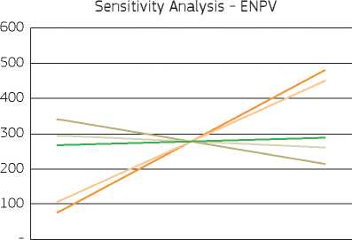
40% 60% 80% 100% 120% 140% 160%
Change in variable
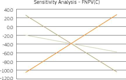
40% 60% 80% 100% 120% 140% 160%
Change in variable
- Investment cost
- O&M costs
- Incremental gas flows
- CO2 price
- Fuel purchase costs
The estimated elasticity of the ENPV and FNPV(C) with respect to the different project variables is shown in the table below.284
|
Variable |
ENPV elasticity |
FNPV(C) elasticity |
|
Investment cost |
-0.46 % |
-3.33 % |
|
O&M costs |
-0.12 % |
-0.99 % |
|
Incremental gas flows |
1.45 % |
3.41 % |
|
CO2 shadow price |
1.23 % |
- |
|
Fuel costs (border prices) |
0.08 % |
- |
The incremental gas flow transmitted by the new pipeline is the most critical variable for the socioeconomic viability. However, the ‘switching value' is relatively high: the ENPV would drop to zero if the volume of the incremental gas flows decrease on average by 69 % over the entire reference period, which does not appear to be very likely. Also, a pessimistic scenario is analysed, where investment costs would be 30 % higher than currently budgeted, while demand and the shadow price of CO2 would be 20 % lower than in the assumed base-case scenario. Under this pessimistic scenario, the ENPV would still be positive (EUR 104 million), with a 9 % ERR. Therefore, it can be concluded that the project should also remain economically viable under reasonably adverse conditions.
As regards the financial profitability of the investment, investment cost and incremental demand are the most critical variables. The FNPV(C) (which is estimated to be negative) would become positive in case the savings in investment costs exceeded 30 % or incremental gas throughput increased by more than 29 % on average over the reference period. The values indicate that the investment would most likely have a negative NPV, so supporting the project with an EU grant appears justified.
Based on the results of the sensitivity analysis and taking into account uncertainties related to aspects not directly reflected in the CBA calculations, a risk matrix was prepared in order to identify possible risk prevention and mitigation measures.
|
Risk description |
Probability* (P) |
Severity* (S) |
Risk level* (=P*S) |
Risk prevention / mitigation measures |
Residual risk |
|
Demand & supply risks | |||||
|
Significant shortfall in demand for transmission capacity |
B |
III |
Moderate |
Projected incremental gas flows based on the results of ‘open season’ procedures. Current economic downturn and protracted low price of EU carbon allowances are also factored in. Function in charge: promoter. |
Low |
|
Supply risks: implementation delays of new LNG terminal and expansions of UGS facilities |
C |
III |
Moderate |
Project implementation units of different projects to liaise with, and under the supervision of, the Ministry of Economy. Incremental project demand can also be met by flexibility in current long-term gas import contract (where maximum annual quantity is reportedly 115 % of annual contract quantity). Function in charge: Ministry of Economy. |
Moderate |
|
Financial risks | |||||
|
Investment cost overrun |
C |
III |
Moderate |
Cost budget based on ‘reference class forecasting’ to correct possible optimism bias. Publication of contract notices in the Official Journal of the EU to ensure wider competition. Function in charge: promoter. |
Low |
|
Late availability of EU grant co-financing |
B |
II |
Low |
Involve JASPERS technical assistance early on in the project cycle. Pre-financing of EU grant to be arranged by the promoter. Function in charge: Ministry of Regional Development and promoter. |
Low |
|
Weak profitability to jeopardise debt service |
B |
I |
Low |
Gas transmission activity is regulated to ensure cost recovery. Tariffs are adjusted by the regulator to give an adequate financial return to the operator in the medium term. Function in charge: National Energy Authority. |
Low |
|
Implementation risks | |||||
|
Problems with land purchase and acquisition of rights of way |
B |
II |
Low |
The project is part of the list of national strategic infrastructure enshrined in the new Energy Act for which facilitated land rights procedures are foreseen. |
Low |
|
Unforeseen technical problems during works |
B |
II |
Low |
Difficult ground conditions (e.g. river crossing, wetland, forest) to be analysed at concept stage. Final pipeline alignment to minimise difficulties. Function in charge: promoter. |
Low |
|
Delays related to extension of tender procedures |
C |
III |
Moderate |
Promoter’s procurement division to be supported by specialised technical assistance. Appropriate time contingencies to be factored in into the project schedule. Function in charge: promoter. |
Low |
|
Environmental risks | |||||
|
Negative impacts on protected areas (Natura 2000) |
A |
II |
Low |
‘Horizontal directional drilling’ technique to be adopted to prevent open excavations generating significant impacts; also, construction works to be banned during the fauna’s reproductive season. Function in charge: contractor. |
Low |
|
Unexpected methane emissions from pipes |
B |
II |
Low |
Use of L485MB steel pipes with wall thickness up to 17.5mm and cathodic protection against corrosion. Function in charge: contractor. |
Low |
* Evaluation scale: Probability: A. Very unlikely; B. Unlikely; C. About as likely as not; D. Likely; E. Very likely.
Severity: I. No effect; II. Minor; III. Moderate; IV. Critical; V. Catastrophic.
Risk level: Low; Moderate; High; Unacceptable.
The results of the sensitivity and risk analyses indicate that the project overall risk level is low to moderate. Also, the measures put in place to prevent the occurrence of the identified risks and/or mitigate their adverse impact should result in a lower residual risk. The probability of the project failing to attain its targeted objective at a reasonable cost can be considered to be marginal. Therefore, the residual project risks are deemed to be fully acceptable and probabilistic risk analysis was not carried out in this particular case study. In the practice, however, it is common that large energy investments undergo a probabilistic risk analysis.
The EU policy framework for broadband investments is the Digital Agenda for Europe and the Industrial Policy Update, which includes a new initiative for digital entrepreneurship as part of the Entrepreneurship 2020 Action Plan. While there is no standardised definition of broadband285, the Digital Agenda foresees the following by 2020:
• all Europeans have access to much higher Internet speeds of above 30 Mbps;
• 50 % or more of European households subscribe to Internet connections above 100 Mbps.
All-encompassing nation- and Europe-wide access to (high-speed) broadband infrastructure is considered essential for a digital economy to contribute towards stimulating social and economic cohesion and as such is one of the priorities of the cohesion policy. Major projects will support large investments in broadband in all Member States and regions, and in particular rural areas, by pursuing investment priority 2a286. The priority is on next generation access networks (NGA), i.e. networks that are capable of delivering broadband access services with enhanced characteristics (i.e. with speeds above 30 Mbps)287.
Investments may concern both the passive (e.g. cable, optical fibre, antenna, etc.) and the active (e.g. router, hub, switch, etc.) components of the infrastructure, including fixed and wireless access solutions. They usually address the extension or upgrade of the regional backbone/backhaul network and/or the area networks, but can also address the last-mile connections. Compliance with the EU State aid rules normally needs to be formally assessed, except for certain categories of aid that are presumed to be compatible with the internal market, provided certain conditions are met, pursuant to the General Block Exemtion Regulation288 (GBER).
A selective list of policy documents for the broadband sector is provided in the box below.
The Digital Agenda for Europe
The Digital Agenda for Europe - Driving European growth digitally (Mid-term Review)
Telecom Single Market Connecting Europe Facility
European Broadband: investing in digitally driven growth [COM(2010) 472]
Better access for rural areas to modern ICT [COM(2009) 103 final] and Commission Staff working document [SEC(2009) 254 of 3.3.2009]
Future networks and the Internet [COM(2008) 594 final]
Bridging the Broadband Gap [COM(2006) 129]
Mobile broadband services [COM(2004) 447 final]
The eEurope 2005 action plan: an information society for everyone [COM(2002) 263 final]
A European Information Society for growth and employment [COM(2005) 229 final]
Guide to High Speed Broadband Investment
EU Guidelines for the application of State aid rules in relation to the rapid deployment of broadband networks Thematic Guidance Fiche for desk officers enhancing access to and use and quality of ICT high-speed broadband roll-out
Broadband investments need to be seen within the greater context of a broadband plan consistent with the priorities set within the Digital Growth Strategy developed, for instance, within the national/regional Smart Specialisation Strategy.
Both the NGN plan and the Digital Growth Strategy constitute ex-ante conditionalities289 (preconditions to be met) enabling the use of EU funds.
Good planning of specific broadband investment that pursues the goals a broadband plan requires the context analysis of the following elements:
• relevant socio-economic issues that characterise the territorial context and affect demand, e.g.: ageing, education, income, level of information and communication technologies (ICT) training/skills, employment status, etc.;
• technical conditions, including a mapping of current broadband coverage, topography, population density, technological alternatives, prospective up-take rates and bandwidth availability;
• market: broadband investments shall primarily come from commercial investors, so it is important that public funds are used in this sector to complement and not to substitute the investments of market players. The mapping of future private investments over the next three years constitute a key element to avoid the displacement of market investment. User requirements need to consider the future development of public and private services over the medium/long term.
Table 6.1 Presentation of the context: Broadband sector
|
Information | |
|
Socioeconomic- trend |
- National and regional GDP growth - Income disposal - Demographic projections - Employment status - Level of education - Level of ICT training and skills |
|
Political, institutional and regulatory factors |
- Reference to the EU Digital Agenda - Reference to national/regional digital growth strategic policy framework - Reference to national/regional next generation networks plans - Availability of regional incentives for future investments into broadband infrastructure |
|
Technical conditions |
- Topography - Users’ density - Presence of existing Infrastructure - Level and quality of existing services - Bandwidth availability |
|
Market conditions |
- Current market size and future investment - Competition level (market share of operators) - Users’ needs (market trends, services offered, future requirements, etc.) - Users’ habits and behaviours regarding Internet usage |
Source: Authors
The main objective of broadband investments is to promote sustainable socioeconomic development and growth through an increased coverage and take-up of broadband services. Intervention is needed when there is no sufficient presence or access to adequate infrastructure, resulting in high prices and/or low quality of services.
In more detail, broadband investments generally aim at:
• improving access to Internet and e-services for households;
• developing new professional opportunities for enterprises;
• driving innovation (new and existing businesses);
• ensuring equity of access to broadband in rural areas and reducing the digital divide;
• increasing productivity for businesses through the use of ICT;
• strengthening development and growth of business start-ups;
• promoting efficiency of the public services through e-government;
• facilitating the provision of reliable e-health, e-education, e-learning, e-commerce, e-culture services;
• strengthening competition in the telecommunication services market.
Project objectives should be always linked to the specific objectives of the EU Digital Agenda and the national/regional ICT policy framework strategy. When feasible, it is also recommended to specify the contribution of the project to the achievement of the OP priorities through the use of indicators290.
The focus of broadband investments concerns:
• network coverage expansions: e.g. projects deploying fibre or cable access networks, as well as high speed mobile access and related support infrastructures to areas that are currently not covered by any access;
• network quality improvements: if the existing quality network is poor and therefore impeding service uptake, the deployment of a higher quality is likely to increase the uptake rate in the area. For instance, in the case of fibre-to-the-home (FTTH) deployment in areas with an existing copper (DSL) network, the FTTH deployments enable much higher broadband access speeds that, in turn, increase the penetration rate of those digital services that require a high bandwidth (e.g. video streaming).
As already mentioned, investments in broadband may comprise both the passive infrastructure and the active components of the network (technology). Passive components291 consist of the physical infrastructure over which information is transmitted, including dark fibre292' Active components include the technological equipment needed to encode the information into signals to be sent over the infrastructure (e.g. transponders, routers and switches, control and management servers).
The technical identification of the project should include a description of:
• the implementation area. This should be supported by maps, indicating the target areas for the intervention and their characteristics (level of presence of actual and targeted broadband transmission speeds and services);
• the network architecture and design, the topology assumptions and the reasons behind it (e.g. the geography of the region, the services finally delivered etc.);
• the design standards and specifications of each project element (e.g. network management centre, fibre optic networks, backbone/distribution nodes, etc.).
The project promoter should specify how the identified technical solution will meet the requirements to reuse, where possible, existing infrastructures, provide open access to both the physical infrastructure and the active equipment and respect the principle of technology neutrality. In particular, the outcome of the mapping exercise with the identification of black, grey and white areas shall be presented vis-a-vis the scope and location of the project. In addition, to identify a broadband project also means to define its institutional set-up, as briefly illustrated in the box below.
According to the latest update of the Commission’s Guide on High Speed Broadband Investment, four levels of involvement of the public sector can be identified, in terms of engagement into investment models to take vis-a-vis the market, the citizens and the businesses in the region.
Public-run municipal network model: the public authority (PA) builds and operates a broadband network (mostly the physical, more rarely the active infrastructure),which may take place in collaboration with the market (PPP) but the ownership of the network remains with the PA. It is sometimes referred to as public design, build and operate (DBO).
Private-run municipal network model: the PA procures the building, but keeps the ownership of of the passive infrastructure, but leaves the operation of the active layer to a private actor that provides wholesale services to retail providers, under an Indefeasible Right of Use (IRU) of, for example, 20 years. This is sometimes referred to as public outsourcing/concession.
Community broadband model: the broadband investment is done as a private initiative, in a so-called bottom-up approach. The role of the PA in this case is to provide support in the form of co-financing, but also of counselling, right-of-way (RoW) granting, regulation and coordination with other infrastructure deployments and access to points of presence, such as major public data centres.
Operator Subsidy(Gap-funding) model: the public authority (PA) does not intervene, limiting itself to subsidising one market actor (typically a major telecom operator) to upgrade its infrastructure. Both passive and active infrastructure are owned and managed by the operator. Risks associated with building new infrastructure and attracting sufficient customers are borne by the recipients of the funding.
Source: European Commission (2014)
Finally, the implementation of any broadband investment should be justified against a set of feasible alternative options allowing the achievement of the same objective (see section 6.6).
The role of demand analysis under the conditions of the European Digital Agenda targets (Europe-wide and nationwide, all-encompassing, full coverage for all inhabitants; minimum thresholds, strict time line for achievement, etc.) is quite different if compared to other infrastructure projects.
Demand analysis is required in order to find out the level of current and prospective demand and to identify which areas and to what extent these requirements can be satisfied through normal market dynamics and those areas which will require some form of public intervention.
Often the question is not whether broadband infrastructure investments should serve those underserved regions that display high actual demand first and those with low demand later (or the other way round), but what actual and foreseeable demand can be discovered in order to make sound decisions for project financing. In this context, the results of demand analysis do not lead to a ranking of projects because eventually all underserved areas and regions will have to be covered by broadband, according to the European policy priorities regarding broadband and Digital Europe.
In this context it must also be kept in mind that European broadband infrastructure investments do not only aim at meeting the current existing demand, but at satisfying and possibly also creating potential demand for services in the future. Consultation with users both in the public and private domains and consideration about technological development and future needs are key aspects to properly size the requirement over the long term, taking into account relevant EU and national aims in the field.
That said, demand forecasts, in terms of expected number of users, are certainly essential to further calculate both the financial and the economic performances of the project (see below).
When forecasting demand for broadband investments, different inter-related factors affecting the take-up rate of digital services need to be taken into account (see Table 6.2).
Table 6.2 Factors influencing demand
|
Factors | |
|
Demand issues |
Socioeconomic conditions: higher standards of living and growing economies are usually associated with a higher use of the Internet. |
|
Digital education and skills: the higher the digital skills of the population, the more likely the use of digital services. | |
|
Geographical and demographic features: in urban/metropolitan areas there is already a wide use of digital services because of favourable market conditions, while the majority of unmet demand for broadband in Europe is in rural areas. In this regard, local communities can play a very important role in driving demand for new services and in some cases providing part of the investment needed. | |
|
Demand aggregation: aggregation of demand for digital services from the side of public authorities (local government, libraries, hospitals, schools, etc.) and the local community (business associations, civil communities/ groups, etc.), generally helps to make the project financially stable over the medium-to-long terms as it secures the use of the infrastructure for the provision of these services. | |
|
Affordability and users’ willingness to pay: capacity and service availability have to consider users’ (households, businesses and public institutions) actual ability/willingness to pay for them.293 Perspective for future demand crated by new infrastructure: structural developments. | |
|
Supply issues |
Capacity and quality of the network/services provided: the take-up of digital services depend on: the infrastructure endowment that can be used for delivery of digital services, the limitations in the quality of services currently provided or services not available in the region, and the level of access to data transmission services. This should equally be compared with estimated future bandwidth and service requirements. Competition level: price-sensitive consumers’ willingness to pay is directly related to competition: the higher the number of operators existing in the market and the variety of services offered, the lower the prices. Additionally, it is recommended that the tariffs paid by the end-user are analysed to see if they would allow for the profit margin that last-mile operators normally expect on the market. Different models of investment allow different degrees of competition.294 |
Source: Authors
The demand analysis should present both current and future demand. The analysis of the current demand should be based on the inventory of the existing demand potential as well as market conditions by mapping the broadband network. This requires presenting the type, scope and quality of existing infrastructure and relative services provided, as well as having a pricing policy in place and future plans.
Given the existing market situation, and considering all the factors affecting demand, forecasts should be estimated by referring to national or international benchmarks of digital service take-up.
The methodology adopted to forecast demand should be clearly explained, with particular reference to the assumptions made on the following:
• expected growth rate during the project horizon;
• degree to which one can expect supply to create demand, as is often the case in infrastructure provisioning;
• future types of services and an analysis of the required bandwidth;
• anticipated structure of revenues generated by the project;
• anticipated level of tariffs and the role of the national regulator as regards price control;
• anticipated market share.
Broadband investments can either aim to provide wholesale services only, retail services (e.g. in the case of a public administration network), or a combination of both. In the first case, demand analysis should be conducted from the point of view of the project users (last-mile network operators); in the second case, from the point of view of the final users. Given that demand from last-mile network operators depends on the demand from final users, such as individuals, businesses and public institutions, it is however common to analyse demand at both levels.
The demand analysis results should therefore be presented in terms of increased coverage, take-up and use (intensity, quality) of digital services, preferably distinguished between the following:
• commercial operators that will obtain wholesale access to the infrastructure and types and features of the digital services provided;
• number of people and households benefiting from the project: in total, as a percentage of the national/regional population, and broken down by municipality (and/or other administrative units) and by urban/rural areas;
• businesses and public institutions making use of digital services.
As regards the relevance of option analysis in the context of European broadband projects, the initial remarks in section
6.5 (demand analysis) apply here as well. Option analysis should be carried out in order to help design the best-suited broadband projects in a given regional environment. However, the results of option analysis do not decide on the provision of broadband as such. Option analysis might further underscore the necessity of broadband deployment, but cannot lead to ‘no broadband', because the European policy goals demand full broadband coverage in the European Union.
The baseline for the option analysis, a scenario without the project, should be discussed by presenting any adverse impact, if quantified as relevant. A scenario without the project usually concerns an option without any infrastructure at all. Alternative options should be analysed and compared with each other on the basis of the following dimensions:
• strategic: compliance and fulfilment of EU objectives and national strategies; socioeconomic impact (who would benefit from the project); scope of intervention (phasing, division into sub-projects, etc.);
• technological: adequate number of different technological alternatives, such as network architecture, dimensioning and topology, hierarchical structure, network transmission medium and protocol, construction of optical cabling or wireless routes, ducting and cable type, in order to maximise the coverage, up-take and sustainability (future-proofed) of the network solution;
• institutional: showing the advantages and disadvantages of alternative investment models for the implementation, indicating which one is best suited for the project promoter, such as in-house management; outsourcing; setting up a special purpose vehicle; separation of construction and operation of the network into two tenders (concession); design-build-operate-transfer (DBOT);
• environmental: observance of environmental quality standards, the potential effect on Natura 2000 sites, etc.;
• financial and economic: project costs and revenues/benefits;
• societal: enabling more and better participation in social life
Once all the feasible options are shortlisted, it is recommended that a simplified CBA is undertaken to rank and select the most optimal solution.
In the case of broadband investments, the passive components of the network (i.e. the permanent physical infrastructure such as copper, fibre and coaxial cable networks, antenna towers) are typically characterised by high capital expenditure, low operational expenditure and limited economies of scale. Furthermore, physical infrastructure is highly local, hard to duplicate and inherently subject to regulation because it most often constitutes a natural monopoly. On the other hand, active equipment (i.e. the application technology installed on the passive infrastructural components, such as routers, transponders, switches, control and management servers, gateways, access points) is characterised by high operational expenditure, economies of scale, and is subject to selective regulation (e.g. regulated, mandatory bit-stream access, which is becoming more and more important in the context of NGA/NGN but must, in most cases, be implemented in active components).
In terms of sources of financing, broadband investments are suitable for delivery through either financial instruments or grants, or a combination of both. In the former case, leverage resources and increased efficiency and effectiveness gains, due to the revolving nature of funds, can give access to a wider spectrum of financial tools for policy delivery and attract private sector support (and financing) to public policy objectives (see box).
In the new programming period the Connecting Europe Facility will devote a limited budget to financing high speed broadband infrastructure. The Connecting Europe facility will operate through a credit enhancement mechanism providing better conditions to loans, guarantees and project bonds issued by the European Investment Bank. The logic behind it is risk sharing, whereby the European Commission and the EIB will join forces to take more risk and improve the credit rating of specific projects that otherwise would find it more difficult to attract investors.
The Connecting Europe Facility is open to contributions from Member States and regions, in particular from European Structural and Investment Funds. Such contributions, which must be geographically ring-fenced (i.e. could only be spent in a MS / region making the contribution) would benefit from the high leverage effect of CEF financial instruments and thus could help maximize the impact of public intervention.
Projections of O&M costs shall be split in fixed and variable costs. Typical operating cost items of broadband investments include Internet traffic and interconnection charges, energy consumption, maintenance costs, and technical and administrative personnel costs. In the case of projects where costs are divided between the owner of the infrastructure and the operator, such a division shall be clearly described.
In most cases, EU-funded broadband projects are designed as wholesale projects. Therefore, revenues should be calculated based on the services provided by the wholesale operator and not against the tariff paid by the final users. Typical sources of revenues are:
• data transmission service fees;
• network connection fees;
• colocation/equipment hosting services fees;
• infrastructure rental revenues, including dark fibre rental, ducts rental, masts rental.
The above categories of revenues should be based on a clearly explained tariff policy. It should, in particular, indicate:
• the benchmarked prices (in case no national benchmark exist, provide international comparison), and
• if the national regulator has been consulted on the tariff setting methodology.
The economic literature suggests that a large number of socioeconomic benefits are associated with broadband coverage and the upgrade of digital services. Examples of benefits that are usually identified are: time savings for Internet browsing, getting more people online, making best use of network capacity, improving micropayment systems, extending the reach of smart solutions, reducing the opportunity cost of providing goods and services via Internet, equity, ubiquity, improved competition, cost savings for the public sector, etc. In particular, an increased use of e-commerce services, especially in rural disadvantaged areas, is seen as a main driver towards economic growth and reduction of territorial disparities and social exclusion. The availability of a state-of-the-art infrastructure is also a key element to improve the attractiveness and competitiveness of an area and its overall competitive edge and can help in reversing the trend of relocation of economic activity and depopulation.
Table 6.3 provides a standardisation of types of economic benefits and relative methodologies for evaluation, which are discussed in more detail in the following sections.
While the economic benefits of broadband investment are widely reported and discussed in the literature, problems nevertheless exist in finding a single, widely accepted methodology to value these benefits in monetary terms, owing to the complexity of the industry. As a consequence, for the main types of benefit (i.e. increased take-up of digital services and improved quality of digital service, see Table 6.3), different evaluation methods are proposed because all are considered acceptable from a methodological point of view.
In addition, while the macroeconomic link between broadband investments and GDP growth is widely recognised and acknowledged, a microeconomic approach to benefit estimation is adopted in this guide. With this approach, the effects on national or regional growth are excluded and replaced by microeconomic estimates as detailed in this chapter. This approach differs from and should not be used together with the methodology for calculating the economic return of coverage expansions looking at the effect on GDP growth.
Table 6.3 Benefit evaluation of broadband investments
|
Economic benefit |
Type |
Valuation method(s) |
|
Increased take-up of digital services for households and businesses |
Direct effect |
- Stated preferences - Travel cost - Benefit transfer - Local gross value added |
|
Improved quality of digital service for households and businesses |
Direct effect |
- Stated preferences - Travel cost - Benefit transfer - Local gross value added |
|
Improved provision of digital services for public administrations |
Direct effect |
- Cost saving |
Source: Authors
A typical (important) benefit that is not included in the list, largely because of a financial nature, are the operational efficiency gains (O&M cost savings) that can be the sole aim of some business-driven network/service modernisation projects. While these projects may lead in some cases to some quality improvements, and also reduced CO2 emissions, the basic rationale typically lies in reducing the operation and maintenance costs of the provider. A typical example is the modernisation of Global System for Mobile Communication (GSM) and third-generation cell-phone technology (3G) networks, where the trend is to move from having separate network equipment for GSM and 3G networks to a single radio access network design, whereby these same services are provisioned by much less active equipment, resulting in lower O&M costs. Therefore the benefit estimation of operational efficiency gains, to a large extent, coincides with the results of the financial analysis.
Finally, in respect to energy consumption, broadband investments are expected to have a neutral or positive impact on CO2 emissions. This comes from the consideration that although ICT networks consume energy, one expects that they will significantly contribute to a reduction of travelling, thereby offsetting the consumption at a minimum. However, it is not yet clear as to what extent new and powerful means of information and communication also generate new demand for the transportation of goods and people with the implication of increased consumption of transport energy. The research base today is not mature enough to measure the net effect of broadband investment on the environment and it is therefore recommended, until relevant studies become available, to discuss this benefit in qualitative terms rather than value its impact in the CBA model.
This benefit arises with respect to projects aimed at both network coverage expansion and network quality improvements.
The methodology for benefit evaluation relies on the concept of WTP for the new users (distinguished between households and businesses) of the digital services.
In the case of competitive markets, the price actually paid by households and businesses for subscription to broadband access (usually in the form of a fixed charge per month) can be used as a proxy of WTP. In other words, the amount paid in subscription charges provides an indication of the value of digital services to consumers. The operational step for the benefit evaluation consists of multiplying the number of households and businesses additionally connected by the expected average revenue per user over the time horizon of the analysis295' Then, in the case of investments designed as wholesale services only, a pro rata factor should be applied to take into account the fact that only part of the benefit to end-users can be attributed to the project.
For the majority of broadband projects, and specifically in the case of regulated prices, it is however reasonable to assume that market prices do not adequately reflect users' WTP, which is expected to be greater than the price actually paid because of the perceived productivity gains (time and cost savings) to customers. In such cases, the WTP must be recalculated together with the following methods, which are mutually exclusive for the same group of users296:
• stated preferences, for instance contingent evaluation or discrete choice experiments, to directly measure the value attributed by users to the applications used over the connection. The disadvantages of this method are that it can be time and resource consuming;
• travel cost: time and cost (e.g. fuel) savings deriving from the use of online services, which replace the need to physically reach a given facility, are estimated on an annual basis in order to incorporate the productivity gains achieved by customers. Although very practical, this method requires a large amount of data that cannot always be available to the project promoter;
• benefit transfer: the result calculated in previous studies is transferred to the project context. In this respect, however, careful judgement is required to determine whether the results are transferable or what adjustments need to be made to make them useful for the project under assessment;
• the local gross value added can be used to estimate the benefit of additional broadband take-up by businesses. The empirical literature suggests, in fact, that productivity gains arise from broadband take-up. The method for benefit evaluation consists of estimating the percentage rise in the expected GVA per employee as a result of the project. While being supported by empirical evidence, this approach is, however, subject to the potential benefit of being double-counted due to the difficulty of measuring the share of GVA rise that can be attributed to the project only.
In light of the constraints each method presents, the benefit transfer seems the most practical, and less costly, approach. It is therefore suggested to always refer to the international literature as a data source where estimated values can be transferred. For a review of selected studies see the reference section.
The quality of the service is improved when the broadband network is upgraded to enable a higher performance (i.e. higher download speeds, reliability and upload speeds). Typical project examples are the deployment of backbones, such as submarine cables to replace satellites, for instance providing backhaul traffic, or the deployment of fibre-based fixed lines or long-term evolution (LTE)/fourth generation (4G) access networks to improve the DSL or 3G-based broadband access networks. The main benefit is produced when the technological upgrade is such that there is a substantial shift from basic to NGA broadband.
As regards assessing the economic return while the service to be enabled already exists on some level, the benefit needs to be corresponded with the increased quality. This calls for a service-based approach, i.e. to investigate the additional possibilities enabled by higher quality services and their productivity gains. Productivity gains may consist, for example, of,lower consumers' costs in using specific applications, the cost saving for an organisation adopting cloud-based services or the Internet of Things, or the increase in value-added in product design or service delivery, or a more targeted advertising provided by applications based on the exploitation of big-data, social networks, etc.
The methodological framework to estimate the WTP for improved quality of digital services follows the same logic as depicted in the previous section. However, care should be taken to ensure that the benefit assessment is carried out in incremental terms so as to measure what consumers would be additionally willing to pay for improvement. In other words, in case of using end-user prices as a proxy, the net benefit is given by the difference between future broadband subscriptions over the current ones. Again, given the difficulties of empirically estimating a WTP that incorporates productivity gains to customers, it is suggested that the benefit estimation is based on data taken from the international literature and, when applicable, adapted to the project context, depending on the project entity, location and scope.
A project aimed at network/service coverage expansion or quality improvements can facilitate the adoption of e-government services, leading to better public service provision and cost savings. For example, the establishment of a fibre-based broadband network may see the government improve and broaden the range of web services for which it is responsible.
The method for benefit evaluation consists of estimating the annual cost savings on the regional/local government expenditure.
In this regard, if project-specific data is not available, the anticipated figure for e-government savings could already be available within the country, probably in an e-government strategy. The benefit realised by the project can therefore be derived as a percentage of the overall target estimated in the region's strategy. This can be estimated by taking into account the relative ‘weight' of the project within that strategy (e.g. on the basis of the share of total households affected by the project). Recognising, however, that not all countries or regions have developed strategies or quantified the savings, a possible means of estimating the project-specific e-government savings is proposed in JASPERS 2013.297
In addition, these projects can facilitate the provision and use of e-services in the different sectors of public expenditure, including health, education, culture, etc. In the context of the major projects, health care is a key sector that is potentially affected. The main benefit from e-health relates to productivity gains in service provision. These unfold when adopting digital applications that:
• improve the capability of patient, clinical and practice management systems to support key electronic information flows between care providers;
• provide datasets that summarise a consumer's key health data and their current state of health, treatments and medications;
• encourage the development of specific tools that improve the quality of clinical decision-making and can reduce adverse events and duplicated treatment activities;
• implementing electronic health records (EHRs), which provide consumers with access to their own consolidated health information and provide care providers with a means of improving the coordination of care.
Again, the method for benefit evaluation consists of estimating the annual cost savings on the regional/local health care budget.
When carrying out the sensitivity analysis, it is recommended to test the following variables:
• investment cost (as disaggregated as possible);
• the anticipated time of usage/lifetime of infrastructure;
• O&M costs (as disaggregated as possible);
• expected demand for services;
• anticipated level of tariffs from the national regulatory authority;
• anticipated market share;
• revenues from different categories of services (as disaggregated as possible);
• unit WTP for households from increased broadband availability or quality or, alternatively, value of time (as relevant);
• unit WTP/ gross value added for businesses from increased broadband availability or quality;
• e-government savings and e-health savings.
Through the sensitivity analysis the most critical variables can be identified. On this basis, detailed qualitative risk assessment must be carried out, typically by assessing the risks presented in the following table.
Table 6.4 Typical risks in broadband projects
|
Stage |
Risk |
|
Context and Regulatory |
- Change of orientation of the strategic policy - Change in excepted behaviour of future private investors - Change in regulations in the retail market - Unsuccessful State-aid application |
|
Demand |
- Lower than estimated service take-up from retail and/or wholesale providers - Low investments in last-mile network by service providers - Low take-up by end-users from service providers |
|
Design |
- Capital expenditure underestimation - Operational expenditure underestimation |
|
Administrative |
- Risk of not obtaining required property rights |
|
Procurement |
- Delays in project public procurement process |
|
Construction |
- Investment cost overruns - Implementation delays |
|
Operation |
- Loss of key personnel during project operation - Increase in O&M cost |
|
Financial |
- Insufficient committed funding on a national/regional level during the operational phase |
Source: Adapted from Annex III to the Implementing Regulation on application form and CBA methodology.
3.20
The scope of the broadband project involves the construction of a fibre-based regional backbone and distribution network infrastructure in a region with 5.25 million inhabitants that have a currently low penetration of broadband services. The project will allow for an important expansion in the provision of two categories of services to households and businesses (in particular SMEs): basic broadband and next generation access (NGA)298. This will allow a considerable improvement to the speed and quality of broadband services. The country's telecommunication's market is characterised by moderate competition with broadband being accessed predominantly through traditional copper infrastructure, mobile subscriptions (2G/3G) and cable connections (35 %; 30 % and 25 % respectively). Over 50 % of broadband connections are offered at a speed of between 2 and 10 Mb/s and the share of high-speed connections (at least 30 Mbps) is lower than the EU average.
The project promoter and the owner of the infrastructure is the regional government, which will tender out the design, construction and operation of the network through a concession contract to a private partner.
The infrastructure consists of both passive and active components. The main technical components defined at a preliminary design stage comprise a fibre optic network with a total length of around 3,600 km, and a total of 180 network nodes, repartitioned between the backbone and distribution network. To reduce the cost of the project and avoid duplications, it was already foreseen at preliminary design level that the final design of the new infrastructure to be carried out by the selected private partner shall incorporate (lease, e.g. indefeasible rights of use, for the project duration) already existing telecommunication infrastructure belonging to operators active in the region.
The project promoter will ensure that retail providers have open and non-discriminatory access to the infrastructure. Last-mile infrastructure is not part of the project. To confirm that sufficient demand exists from last-mile operators, letters of intent have been signed with the majority of service providers in the region.
The project objectives are aligned with the goals of the Digital Agenda for Europe in terms of access to basic broadband, next generation access and the country's National Strategy for the Development of the Information Society.
The general objective of the investment is to help to eliminate the digital divide related to the availability of basic broadband in areas where this is currently not provided due to market failures, and to lower the investment barrier for NGA services.
More specifically, the project aims at the following:
• households in general: improving access to e-services (e-commerce, e-banking), better access to information, development of new professional opportunities for skilled residents (e.g. teleworking);
• businesses: increasing productivity through the use of ICT (e.g. by a reduction of transportation costs, etc.);
• for government, facilitating the adoption of e-government services, leading to better service and cost savings;
• for the healthcare sector: facilitating the provision of faster and better tailored e-health services.
Other sectors that can benefit from the project in the medium term are the energy sector (smart grids, controlling decentralised energy generation) and the transport sector (multimodal traffic planning).
As a direct result of the project, it is estimated that NGA broadband coverage will increase from 63 % to 75 % of the population (additionally connecting 630,000 inhabitants or 300,000 households). In addition, fixed basic broadband coverage will increase from 80 % to 96 % of the region's population (additionally connecting 840,000 inhabitants or 400,000 households).
The project is well aligned with the goals of the relevant priority axis of the operational programme concerned. Specifically, the project will contribute to the following OP indicators:
|
Result indicator |
OP 2023 target |
Project (% of OP target) |
|
Additional households with basic broadband access |
450,000 |
400,000 (89 %) |
|
Additional households with NGA broadband access |
400,000 |
300,000 (75 %) |
|
Additional enterprises with NGA broadband access |
60,000 |
40,000 (66 %) |
|
Output indicator |
OP 2023 target |
Project (% of OP target) |
|
Increase in the length of fibre optical network |
5,000 |
3,600 (72 %) |
In order to define the areas of intervention, the region was mapped according to the existing level of competition for relevant broadband services, based on a method described in the State aid guidelines for broadband projects299.
The demographic and socioeconomic characteristics of the selected areas were then benchmarked with historic market developments in comparable areas at national and European level, to produce detailed forecasts of project demand. The following main factors were analysed in detail: i) potential increase in take-up of bandwidth; ii) market share potential of project operator; iii) assessment of demand for existing and new e-services from households and businesses (accompanied by estimations of associated bandwidth requirements).
The resulting prognoses were consulted with service providers active in the market, both wholesalers and potential last-mile operators, for a reality check of the initial assumptions. After some final corrections, the following uptake rates were estimated for the end-users of the infrastructure.
|
Cat. |
Broadband uptake in project area (%) |
2018 |
2023 |
2028 |
2033 |
|
Households | |||||
|
I |
New uptake of basic broadband |
20 |
25 |
25 |
25 |
|
II |
New uptake of NGA (where previously zero) |
15 |
35 |
53 |
55 |
|
III |
Upgrade from basic broadband to NGA300 |
15 |
42 |
58 |
58 |
|
Businesses | |||||
|
IV |
New uptake of or upgrade to NGA (from basic broadband) |
50 |
80 |
90 |
90 |
The baseline for the option analysis is an option with no infrastructure. This was deemed as non-compatible with both the national objectives and those objectives set out in the Digital Agenda for Europe. Public consultations with operators resulted in a list of areas where there are no plans to invest in relevant broadband infrastructure in the near future. It was therefore concluded that not implementing the project would lead to an increase in the digital divide (the use of ICT) between the areas identified as non-attractive to the market and the remaining areas of the region. This would result in the digital exclusion of citizens and brain drain, as well as negative competitive effects for local business.
As a first stage, two strategic options were assessed by analysing compliance with the national and EU objectives:
• phasing the infrastructure deployment (splitting the implementation over separate periods of time, initially providing backhaul and last-mile services to only part of the target areas of the region);
• providing backhaul network coverage to the maximum number of households and SMEs.
The phasing of infrastructure deployment was discarded on the grounds of a lower mid-term socioeconomic impact and compatibility with EU objectives. The estimated higher total project costs as well as the technical challenges resulting from a split of the implementation were also assessed as unreasonable. The option of maximising the network coverage was deemed as fulfilling the EU objectives and enabling coverage to the largest number of households and businesses, further leveraging private investments into last-mile network infrastructure.
The option analysis then considered three sets of options concerning different aspects of the project.
• technical alternatives;
• linear infrastructure alternatives;
• business model alternatives.
A number of technical options were analysed in detail for:
• network architecture, dimensioning and topology,
• hierarchical structure,
• network transmission medium and protocol,
• construction of optic cabling routes, ducting and cable type.
The choice of network architecture and topology and its hierarchical structure followed what is generally considered to be best practice for network design. Consequently, the baseline design proposed a two-layer hierarchical design, with a crossover ring topology for the backbone and a star topology for the backhaul network. The final design will take into account the existing infrastructure in the region as much as possible and will be updated accordingly, subject to the approval of the project promoter.
The selection of other network technologies was guided based on the optimisation of capacity and the efficiency of the planned network. The main criterion for the selection was the requirement to ensure that the technologies used could be considered as future-proof, i.e. that they minimise additional investments in case of an increase in demand or capacity requirements. Consequently, the project promoter equally analysed the options of partial upgrading of existing infrastructure as well as the use of satellite technology for the backhaul network. However, these were discarded as they would not meet the long-term requirements of a future-proof network. Fibre was deemed to be the optimal choice to ensure that the objectives of the project were met.
Three public utility infrastructure networks were considered to help to bring down the construction cost by using already existing routes to lay down the fibre:
• scenario A - railway infrastructure
• scenario B - road infrastructure
• scenario C - energy infrastructure.
Variants were compared, based on multiple criteria, such as how well the different options would allow the maintenance of an optimal network design and capacity, potential cost savings, and their technical feasibility and environmental compliance. In this case, the rail infrastructure was assessed as offering the highest potential use of the existing infrastructure, with a comparable cost structure to the road scenario and lower than the energy scenario, it was feasible and would have the least negative impact on the environment, as would the energy scenario. It was ultimately selected as the preferred choice for the construction of the network, as it is technically and economically feasible.
The choice of the operational model for the project was drawn from an analysis between five different management models:
• in-house management,
• technical outsourcing,
• setting up a special purpose vehicle,
• separation of construction and operation of the network into two tenders,
• design-build-operate-transfer (DBOT).
The options were compared, based on multiple criteria such as estimated cost, possibilities for management oversight and audit by regional authorities, operational risk, and the competences of potential private partners. As a result, the design-build-operate-transfer concession model, in which the construction and operation of the network are tendered in one stage, was selected. Under the chosen DBOT model, the public partner (regional authority) will provide for the financing of the investment and be the owner of the assets, and the selected private partner will be responsible for the design, construction and subsequent management and operation of the infrastructure during the concession period, after which the project's infrastructure will be returned to the public partner. The private partner will cash in the revenues from the wholesale services delivered to users (last-mile operators and others) and pay a certain percentage of that income to the public partner as rent for the infrastructure (to be defined in the tender process). A claw-back mechanism will be included in the contract to avoid any over-compensation to the private partner.
The total project investment costs of the selected option were estimated based on best industry and in-house expertise. A cost breakdown is presented in the table below.
|
EUR |
Total project costs (A) |
Ineligible costs (B) |
Eligible costs (C)=(A)-(B) | |
|
1 |
Planning/design fees |
11,000,000 |
0 |
11,000,000 |
|
2 |
Land purchase |
0 |
0 |
0 |
|
3 |
Building and construction |
62,000,000 |
0 |
62,000,000 |
|
4 |
Plant and machinery |
13,000,000 |
0 |
13,000,000 |
|
5 |
Contingencies |
0 |
0 |
0 |
|
6 |
Price adjustment (if applicable) |
0 |
0 |
0 |
|
7 |
Technical assistance |
0 |
0 |
0 |
|
8 |
Publicity |
4,500,000 |
0 |
4,500,000 |
|
9 |
Supervision during construction implementation |
7,000,000 |
0 |
7,000,000 |
|
10 |
Sub-TOTAL |
97,500,000 |
0 |
97,500,000 |
|
11 |
VAT |
20,585,000 |
20,585,000 |
0 |
|
12 |
TOTAL |
118,085,000 |
20,585,000 |
97,500,000 |
With regards to operation and maintenance (O&M) costs, a detailed breakdown by type of cost was prepared as part of the project feasibility study. The owner of the infrastructure will bear the administrative costs related to the audit and oversight, estimated at being in the region of EUR 0.7 million annually (with a gradual increase from EUR 0.3 million in the first year of operation). The costs assigned to the private partner include Internet traffic and interconnection charges, maintenance costs, energy consumption and third-party services (administration and personnel, insurance). This showed that the O&M cost would be about EUR 2 million in the first year of operation, with a gradual increase to EUR 5.4 million in the last years of operation. The increase in costs related to Internet traffic, interconnection charges and energy consumption is linked to the increase in broadband uptake rates and the increase in forecast demand for bandwidth (moving from basic broadband to NGA broadband) over the duration of the project. The replacement of active equipment totalling EUR 9.3 million is planned in years 11-13 after the start of operations and will be covered by the infrastructure operator.
The results of the demand analysis were used to estimate revenues from the three broad categories of wholesale services:
• data transmission services
• lease of infrastructure
• colocation/equipment hosting services.
These revenues have been estimated at about EUR 2.2 million in the first year of operation with a gradual increase to EUR 9 million in the last year of operation. The estimation of financial revenues was based on benchmarked wholesale service prices in areas where relevant wholesale services are provided and set at the level of EUR 30/month for NGA access to businesses; EUR 20/month for NGA access to households and EUR 10/month for basic broadband access. The regulator was consulted on the prices and will continue to monitor their level during the project operation. Revenues from line rental and colocation services were calculated together as a percentage of the revenues from wholesale services, which was estimated at 55 % of the revenues from transmission services during the project duration and reflects the results of surveys on fixed and mobile network operators, which verified the market demand for these services.
The financial and economic analysis of the project is based on the incremental approach. All cash flows are stated in constant EUR and the real discount rates applied are 4 % in the financial analysis and 5 % in the economic analysis. The reference period was set at 20 years, including three years of construction. As the average economic life of the project assets is assumed to be 20 years, a residual value is considered in the last year of the time horizon, reflecting the discounted value of the net cash flows in the remaining years.301
The financial analysis is conducted in a consolidated manner, including the owner and the operator of the infrastructure, without consideration of the internal cash flows between them (rent paid for the infrastructure). The financial profitability indicators calculated for return on investment [FNPV(C) of the project is EUR -68.5 million and the financial rate of return on the investment, FRR(C) is -6.4 %] confirm that the project would not take place without grant support.
The project is subject to the rules on State aid and was therefore notified to the European Commission. After examination by the Directorate-General for Competition the project was found to be compatible with State aid regulations and subsequently authorised. A calculation of discounted net revenue is in principle not necessary for projects when an individual verification of financing needs is carried out in accordance with applicable State Aid rules. However, in this case, national rules required the project promoter to nevertheless undertake this calculation in order to determine the appropriate level of ERDF contribution and avoid overcompensation.
Based on the costs and revenues described in the section above, the estimated pro-rata application of discounted net revenue is 77 % (DIC = EUR 88.7 million, DNR = EUR 20.2 million, see further calculation below). Multiplying the eligible cost (EUR 97.5 million) by the pro-rata application of discounted net revenue and by the co-financing rate of the relevant priority axis of the OP (85 %), the EU grant for the project results in EUR 64 million. The remainder of the investment (EUR 33.5 million) is to be funded by the project promoter and owner of the infrastructure.
The fact that the financial rate of return on national capital [FRR(K) is equal to 0.9 %] is below the discount rate applied and that the financial return on national capital is negative [FNPV(K) is equal to EUR -10.3 million] further shows that the investment aid granted is not over-proportionate.
It needs to be noted here that although last-mile operators were consulted in advance, there is a certain level of uncertainty with regards to the final level of revenues that will be generated by the infrastructure. This was acknowledged in Directorate-General for Competition's State aid decision, which required the inclusion of a claw-back mechanism into the concession contract that would apply in case revenues are higher than originally foreseen302. The State aid decision also includes provisions on the use of the revenues recovered through the claw-back mechanism on the side of the public authorities303.
The sustainability analysis was performed for the project as a whole and shows that based on the assumptions described above the project will not run out of cash during the implementation and operating periods. Sufficient securities were provided by the regional authority as the project promoter that allow there to be sufficient confidence in its capability to co-finance the project.
Financial cash flows and performance indicators of the project
|
12 3 |
4 5 6 7 8 9 10 11 12 13 14 15 20 |
|
Construction |
Operation |
Table 1
EU GRANT
|
Calculation of Discounted Investment Cost (DIC) |
NPV 4% | |||||||||||||||||
|
Investment cost (excluding contingencies) |
mEUR |
-88.7 |
-9.5 |
-36.5 |
-51.5 |
0.0 |
0.0 |
0.0 |
0.0 |
0.0 |
0.0 |
0.0 |
0.0 |
0.0 |
0.0 |
0.0 |
0.0 |
0.0 |
|
DIC / Investment cost cash-flow |
mEUR |
-88.7 |
-9.5 |
-36.5 |
-51.5 |
0.0 |
0.0 |
0.0 |
0.0 |
0.0 |
0.0 |
0.0 |
0.0 |
0.0 |
0.0 |
0.0 |
0.0 |
0.0 |
|
Calculation of Discounted Net Revenues (DNR) |
NPV 4% | |||||||||||||||||
|
Revenues - data transmission services |
mEUR |
46.1 |
0.0 |
0.0 |
0.0 |
1.4 |
2.2 |
2.9 |
3.4 |
3.7 |
4.0 |
4.3 |
4.6 |
4.9 |
5.2 |
5.5 |
5.7 |
5.8 |
|
Revenues - lease of infrastructure and dark fibre |
mEUR |
25.4 |
0.0 |
0.0 |
0.0 |
0.8 |
1.2 |
1.6 |
1.9 |
2.0 |
2.2 |
2.4 |
2.5 |
2.7 |
2.9 |
3.0 |
3.1 |
3.2 |
|
O&M cost - maintenance |
mEUR |
-14.9 |
0.0 |
0.0 |
0.0 |
-0.7 |
-1.1 |
-1.5 |
-1.5 |
-1.5 |
-1.5 |
-1.5 |
-1.5 |
-1.5 |
-1.5 |
-1.5 |
-1.5 |
-1.5 |
|
O&M cost - energy |
mEUR |
-3.7 |
0.0 |
0.0 |
0.0 |
-0.1 |
-0.2 |
-0.2 |
-0.3 |
-0.3 |
-0.3 |
-0.3 |
-0.4 |
-0.4 |
-0.4 |
-0.4 |
-0.5 |
-0.5 |
|
O&M cost - IP traffic |
mEUR |
-13.8 |
0.0 |
0.0 |
0.0 |
-0.4 |
-0.6 |
-0.9 |
-1.0 |
-1.1 |
-1.2 |
-1.3 |
-1.4 |
-1.5 |
-1.6 |
-1.6 |
-1.7 |
-1.7 |
|
O&M cost - labour and administrative costs |
mEUR |
-16.6 |
0.0 |
0.0 |
0.0 |
-0.7 |
-1.0 |
-1.2 |
-1.7 |
-1.7 |
-1.7 |
-1.7 |
-1.7 |
-1.7 |
-1.7 |
-1.7 |
-1.7 |
-1.7 |
|
Replacement cost |
mEUR |
-5.8 |
0.0 |
0.0 |
0.0 |
0.0 |
0.0 |
0.0 |
0.0 |
0.0 |
0.0 |
0.0 |
-3.1 |
-3.1 |
-3.1 |
0.0 |
0.0 |
0.0 |
|
Residual value of investments |
mEUR |
3.5 |
0.0 |
0.0 |
0.0 |
0.0 |
0.0 |
0.0 |
0.0 |
0.0 |
0.0 |
0.0 |
0.0 |
0.0 |
0.0 |
0.0 |
0.0 |
7.6 |
|
DNR / Net revenue cash-flow |
mEUR |
20.2 |
0.0 |
0.0 |
0.0 |
0.2 |
0.4 |
0.7 |
0.8 |
1.2 |
1.5 |
1.9 |
-0.9 |
-0.5 |
-0.1 |
3.2 |
3.5 |
11.2 |
|
ELIGIBLE COST (EC) |
mEUR |
97.5 |
|
Pro-rata application of DNR = (DIC - DNR) / DIC |
77% | |
|
CO-FINANCING RATE IN PRIORITY AXIS (CF) |
85.0% | |
|
EU GRANT ( = EC x PRO-RATA x CF) |
mEUR |
64.0 |
|
FRR(C) |
1 |
2 |
3 |
4 |
5 |
6 |
7| |
8 |
9 |
10 |
11 |
12 |
13 |
14 |
15 |
20 | ||
|
Construction |
Operation | |||||||||||||||||
|
Calculation of the Return on Investment |
NPV 4% | |||||||||||||||||
|
Investment cost (excluding contingencies) |
mEUR |
-88.7 |
-9.5 |
-36.5 |
-51.5 |
0.0 |
0.0 |
0.0 |
0.0 |
0.0 |
0.0 |
0.0 |
0.0 |
0.0 |
0.0 |
0.0 |
0.0 |
0.0 |
|
O&M cost |
mEUR |
-49.0 |
0.0 |
0.0 |
0.0 |
-2.0 |
-2.9 |
-3.8 |
-4.5 |
-4.6 |
-4.7 |
-4.8 |
-4.9 |
-5.0 |
-5.1 |
-5.2 |
-5.3 |
-5.4 |
|
Replacement cost |
mEUR |
-5.8 |
0.0 |
0.0 |
0.0 |
0.0 |
0.0 |
0.0 |
0.0 |
0.0 |
0.0 |
0.0 |
-3.1 |
-3.1 |
-3.1 |
0.0 |
0.0 |
0.0 |
|
Revenues |
mEUR |
71.5 |
0.0 |
0.0 |
0.0 |
2.2 |
3.4 |
4.5 |
5.3 |
5.7 |
6.2 |
6.7 |
7.1 |
7.6 |
8.1 |
8.5 |
8.9 |
9.0 |
|
Residual value of investments |
mEUR |
3.5 |
0.0 |
0.0 |
0.0 |
0.0 |
0.0 |
0.0 |
0.0 |
0.0 |
0.0 |
0.0 |
0.0 |
0.0 |
0.0 |
0.0 |
0.0 |
7.6 |
|
FNPV(C) - before EU grant / Net cash-flow |
mEUR |
-68.5 |
-9.5 |
-36.5 |
-51.5 |
0.2 |
0.4 |
0.7 |
0.8 |
1.2 |
1.5 |
1.9 |
-0.9 |
-0.5 |
-0.1 |
3.2 |
3.5 |
11.2 |
|
FRR(C) - before EU grant |
-6.4% | |||||||||||||||||
|
FRR(K) |
1 |
2 |
3 |
4 |
5 |
6 |
7| |
8 |
9 |
10 |
11 |
12 |
13 |
14 |
15 |
20 | ||
|
Construction |
Operation | |||||||||||||||||
|
National Financing Sources | ||||||||||||||||||
|
Promoter's contribution (Regional Government) |
mEUR |
3.3 |
12.5 |
17.7 |
0.0 |
0.0 |
0.0 |
0.0 |
0.0 |
0.0 |
0.0 |
0.0 |
0.0 |
0.0 |
0.0 |
0.0 |
0.0 | |
|
Calculation of the Return on National Capital |
NPV 4% | |||||||||||||||||
|
Promoter's contribution (Regional Government) |
mEUR |
-30.5 |
-3.3 |
-12.5 |
-17.7 |
0.0 |
0.0 |
0.0 |
0.0 |
0.0 |
0.0 |
0.0 |
0.0 |
0.0 |
0.0 |
0.0 |
0.0 |
0.0 |
|
O&M cost |
mEUR |
-49.0 |
0.0 |
0.0 |
0.0 |
-2.0 |
-2.9 |
-3.8 |
-4.5 |
-4.6 |
-4.7 |
-4.8 |
-4.9 |
-5.0 |
-5.1 |
-5.2 |
-5.3 |
-5.4 |
|
Replacement cost |
mEUR |
-5.8 |
0.0 |
0.0 |
0.0 |
0.0 |
0.0 |
0.0 |
0.0 |
0.0 |
0.0 |
0.0 |
-3.1 |
-3.1 |
-3.1 |
0.0 |
0.0 |
0.0 |
|
Revenues |
mEUR |
71.5 |
0.0 |
0.0 |
0.0 |
2.2 |
3.4 |
4.5 |
5.3 |
5.7 |
6.2 |
6.7 |
7.1 |
7.6 |
8.1 |
8.5 |
8.9 |
9.0 |
|
Residual value of investments |
mEUR |
3.5 |
0.0 |
0.0 |
0.0 |
0.0 |
0.0 |
0.0 |
0.0 |
0.0 |
0.0 |
0.0 |
0.0 |
0.0 |
0.0 |
0.0 |
0.0 |
7.6 |
|
FNPV(K) - after EU grant / Net cash-flow |
mEUR |
-10.3 |
-3.3 |
-12.5 |
-17.7 |
0.2 |
0.4 |
0.7 |
0.8 |
1.2 |
1.5 |
1.9 |
-0.9 |
-0.5 |
-0.1 |
3.2 |
3.5 |
11.2 |
|
FRR(K) - after EU grant |
0.9% | |||||||||||||||||
FINANCIAL SUSTAINABILITY (consolidated)
|
12 3 |
4 5 6 7 8 9 10 11 12 13 14 15 20 |
|
Construction |
Operation |
Verification of the
Financial Sustainability of the Project
EU grant
Promoter's contribution (Regional Government) Revenue
Total cash inflows
Investment cost (including contingencies)
O&M cost
Replacement cost
Income tax (private partner)
Total cash outflows
Net cash-flow
Cumulated net cash-flow
mEUR
mEUR
mEUR
mEUR
mEUR
mEUR
mEUR
mEUR
mEUR
mEUR
mEUR
|
6.2 |
24.0 |
33.8 |
0.0 |
0.0 |
0.0 |
0.0 |
0.0 |
0.0 |
0.0 |
0.0 |
0.0 |
0.0 |
0.0 |
0.0 |
0.0 |
|
3.3 |
12.5 |
17.7 |
0.0 |
0.0 |
0.0 |
0.0 |
0.0 |
0.0 |
0.0 |
0.0 |
0.0 |
0.0 |
0.0 |
0.0 |
0.0 |
|
0.0 |
0.0 |
0.0 |
2.2 |
3.4 |
4.5 |
5.3 |
5.7 |
6.2 |
6.7 |
7.1 |
7.6 |
8.1 |
8.5 |
8.9 |
9.0 |
|
9.5 |
36.5 |
51.5 |
2.2 |
3.4 |
4.5 |
5.3 |
5.7 |
6.2 |
6.7 |
7.1 |
7.6 |
8.1 |
8.5 |
8.9 |
9.0 |
|
-9.5 |
-36.5 |
-51.5 |
0.0 |
0.0 |
0.0 |
0.0 |
0.0 |
0.0 |
0.0 |
0.0 |
0.0 |
0.0 |
0.0 |
0.0 |
0.0 |
|
0.0 |
0.0 |
0.0 |
-2.0 |
-2.9 |
-3.8 |
-4.5 |
-4.6 |
-4.7 |
-4.8 |
-4.9 |
-5.0 |
-5.1 |
-5.2 |
-5.3 |
-5.4 |
|
0.0 |
0.0 |
0.0 |
0.0 |
0.0 |
0.0 |
0.0 |
0.0 |
0.0 |
0.0 |
-3.1 |
-3.1 |
-3.1 |
0.0 |
0.0 |
0.0 |
|
0.0 |
0.0 |
0.0 |
0.0 |
0.0 |
0.0 |
-0.1 |
-0.1 |
-0.1 |
-0.1 |
0.0 |
0.0 |
-0.2 |
-0.1 |
0.0 |
-0.3 |
|
-9.5 |
-36.5 |
-51.5 |
-2.0 |
-2.9 |
-3.8 |
-4.5 |
-4.6 |
-4.8 |
-4.9 |
-8.0 |
-8.1 |
-8.4 |
-5.3 |
-5.3 |
-5.6 |
|
0.0 |
0.0 |
0.0 |
0.2 |
0.4 |
0.7 |
0.7 |
1.1 |
1.5 |
1.8 |
-0.9 |
-0.5 |
-0.3 |
3.2 |
3.5 |
3.4 |
|
0.0 |
0.0 |
0.0 |
0.2 |
0.7 |
1.4 |
2.1 |
3.2 |
4.7 |
6.5 |
5.6 |
5.1 |
4.7 |
7.9 |
11.4 |
28.3 |
The economic analysis is conducted from the perspective of the society that will benefit from an increased broadband connectivity.
On the cost side, the same investment and operating costs used in the financial analysis are applied and corrected where necessary. In this case, corrections to financial prices were made for:
• non-skilled labour component in the investment cost (in particular in the building and construction component), by applying a shadow wage correction factor (CF) to account for the high unemployment level in the project area, correction factor = 0.7;
• taxes (municipal taxes, not related to VAT, to be paid for the use of infrastructure) were removed from the economic analysis (correction factor = 0);
• energy prices in O&M costs, by taking into account the share of taxes and levies paid by industrial customers based on Eurostat data, correction factor = 0.8;
• all other project cost components were left uncorrected, as it was assumed that these are adequately priced on the market, correction factor = 1304.
On the benefit side, financial revenues of the project were disregarded305 306 and instead the project's socioeconomic benefits were estimated by applying proxies for the WTP of users in accordance with the methodology and assumptions presented in the following table. The economic benefits are directly linked to the project objectives and the expected demand of end-users, i.e. local businesses, households and providers of public services such as government and health services.
To take into account the fact that the project does not include last-mile networks and services, the estimated project benefits were allocated in accordance with the project's share of the total costs required to provide the services to the end users (estimated at 50 %). Furthermore, for upgrades from the basic to the NGA broadband category, an 80 % scaling factor has been applied when calculating e-government and tele-health-care benefits to recognise the effect a higher bandwidth has on the type of services that can be provided.
Table 2 Assessment of socioeconomic benefits305
|
Indicator |
Assessment |
|
Benefit 1: Business employee benefits | |
|
Business benefit per employee |
Business benefits are expressed as a percentage increase of local gross value added (GVA) per employee in the private sector for different broadband (BB) services: - new connection to basic BB: 4.5 % rise in GVA per employee - new connection to NGA BB: 6.0 % rise in GVA per employee - upgrade from basic BB to NGA BB: 1.5 % rise in GVA per employee The values proposed are the results of an analysis of productivity resulting from broadband take-up and are based on the available report, which suggests an average potential rise in GVA per person across ‘aspiring’ countries of around 11 %, including the one EU-12307 Member State in the study with a figure of around 6 %. As the project is realised in a country with a similar level of GDP per capita, no further GDP adjustments were applied and the figure was maintained. |
|
Indicator |
Assessment |
|
Figures regarding the GVA rise for other broadband categories have been derived from an International Telecommunications Union (ITU) study that assumes doubling the broadband speed results in 0.3 % rise in GVA308. The GVA rise due to basic broadband is 4.5 % (6.0 % - 5*0.3 %) because it is assumed that the basic broadband speed needs to be doubled approximately five times to reach NGA broadband speeds. Finally, the GVA rise from basic to NGA broadband is calculated as the differential between NGA broadband and basic broadband. This category of benefits is assumed to take four years after project operations have been initiated to fully emerge. Calculated as: GVA value in the region * number of employees connected to basic or NGA broadband as a result of the project * percentage rise in GVA as explained above. Based on the assumption that most businesses newly connecting to broadband services are very small SMEs and in order to apply a conservative assumption, it is assumed that for each enterprise that is newly connected or upgrading its broadband connection, the average number of employees using modern ICT in their daily work is 1. |
Benefit 2: Household consumer surplus
|
Consumer surplus |
Household benefits are expressed in EUR per month and household for different BB services: - new connection to basic BB: EUR 12 per month and household - new connection to NGA BB: EUR 8 per month and household - upgrade from basic BB to NGA BB: EUR 4 per month and household To estimate the level of consumer surplus, the benefit transfer method was applied: estimations of consumer surplus from NGA-types of services were derived from the industry study and were adjusted for differences in income levels and differences in the costs of living (using Eurostat data on GDP per capita in purchasing power standards, PPS). Consumer surplus in USD Consumer GDP Consumer Average based on the study surplus in EUR adjustment surplus adjusted (EUR) EU Country 1 28 21 0.6 12 12 EU Country 2 26 19 0.7 13 EU Country 3 22 16 0.6 10 EU Country 4 17 13 1.0 13 As the speed of broadband connectivity is as important as the range of benefits that can be obtained, the value of EUR 8 per month for basic broadband Internet and a differential of EUR 4 if the consumer switches from basic to NGA broadband was further applied, based on expert knowledge. Calculated as: Level of consumer surplus as set above * number of connected households to basic or NGA broadband as a result of the project * number of months per year * benefit ratio |
Benefit 3: e-government savings
|
e-government savings |
Estimation of savings from e-government was based on the region’s strategy, which states that the implementation of e-government measures (broadband connectivity and e-government services) would result in annual savings of EUR 100 million. This target was then scaled down to only take into account the share of total households connected by the project. Calculated as: Target e-government savings from regional strategy * share of households connected to the network as the result of the project * benefit ratio. |
Benefit 4: Tele-health-care benefits
|
Tele-healthcare savings |
The analysis has made an attempt to apply the benefit transfer method to estimate the savings related to tele-health-care benefits. While available studies confirmed that a high-speed network can yield benefits such as more efficient management and improved health outcomes, the results are preliminary and indicate the need to measure the scale of benefits further. For the purpose of analysis, conservative assumptions were made to estimate tele-health-care savings as a 1-3 % share of the local health budget (1 % in first five years after roll-out and 3 % thereafter) and scaled down to only take into account the share of total households connected by the project. Calculated as: Local health budget * percentage share of households connected to the network as a result of the project (further application of 0.8 scaling factor for new connections to basic broadband and upgrade from basic to NGA) * estimated share in realising the savings (1 % or 3 % as above) * benefit ratio |
Based on these assumptions, the following economic indicators are calculated (see Table 3).
Table 3 Calculation of economic rate of return (ERR) and economic cost-benefit ratio
|
ERR |
12 3 |
4 5 6 7 8 9 10 11 12 13 14 15 20 | ||||||||||||||||
|
Construction |
Operation | |||||||||||||||||
|
Calculation of the Economic Rate of Return |
NPV 5% | |||||||||||||||||
|
Investment cost (excluding contingencies) |
mEUR |
-79.9 |
-9.2 |
-34.2 |
-47.6 |
0.0 |
0.0 |
0.0 |
0.0 |
0.0 |
0.0 |
0.0 |
0.0 |
0.0 |
0.0 |
0.0 |
0.0 |
0.0 |
|
O&M cost (including replacement cost) |
mEUR |
-45.6 |
0.0 |
0.0 |
0.0 |
-2.0 |
-2.9 |
-3.7 |
-4.4 |
-4.5 |
-4.6 |
-4.7 |
-7.9 |
-8.0 |
-8.2 |
-5.2 |
-5.2 |
-5.3 |
|
Residual value of investments |
mEUR |
18.9 |
0.0 |
0.0 |
0.0 |
0.0 |
0.0 |
0.0 |
0.0 |
0.0 |
0.0 |
0.0 |
0.0 |
0.0 |
0.0 |
0.0 |
0.0 |
55.3 |
|
Total economic cost |
mEUR |
|-106.6 |
-9.2 |
-34.2 |
-47.6 |
-2.0 |
-2.9 |
-3.7 |
-4.4 |
-4.5 |
-4.6 |
-4.7 |
-7.9 |
-8.0 |
-8.2 |
-5.2 |
-5.2 |
50.0 |
|
Economic benefits -Business employee benefits |
mEUR |
73.9 |
0.0 |
0.0 |
0.0 |
5.3 |
5.8 |
6.3 |
6.8 |
7.4 |
7.9 |
8.4 |
8.9 |
9.5 |
9.5 |
9.5 |
9.5 |
9.5 |
|
Economic benefits -Household consumer surplus |
mEUR |
82.7 |
0.0 |
0.0 |
0.0 |
3.5 |
5.6 |
7.1 |
8.0 |
8.4 |
8.9 |
9.3 |
9.7 |
10.2 |
10.7 |
11.0 |
11.4 |
11.5 |
|
Economic benefits -e-Government savings |
mEUR |
35.6 |
0.0 |
0.0 |
0.0 |
1.5 |
2.4 |
3.0 |
3.5 |
3.7 |
3.9 |
4.0 |
4.2 |
4.4 |
4.6 |
4.8 |
4.9 |
5.0 |
|
Economic benefits -Tele-health care benefits |
mEUR |
5.0 |
0.0 |
0.0 |
0.0 |
0.1 |
0.1 |
0.5 |
0.5 |
0.5 |
0.6 |
0.6 |
0.6 |
0.7 |
0.7 |
0.7 |
0.7 |
0.7 |
|
Total economic benefits |
mEUR |
197.3 |
0.0 |
0.0 |
0.0 |
10.3 |
13.9 |
16.9 |
18.8 |
20.0 |
21.2 |
22.4 |
23.5 |
24.7 |
25.4 |
26.0 |
26.5 |
26.7 |
|
ENPV / Net benefits |
mEUR |
100.5 |
-9.2 |
-34.2 |
-47.6 |
8.4 |
11.0 |
13.1 |
14.4 |
15.5 |
16.6 |
17.7 |
15.5 |
16.6 |
17.3 |
20.8 |
21.3 |
76.7 |
|
ERR |
14.4% | |||||||||||||||||
|
B/C RATIO |
1.85 | |||||||||||||||||
Despite its low financial profitability, the high economic profitability (ERR: 14.4 %, B/C Ratio: 1.85) makes the project worthy of the support of EU funds.
A sensitivity analysis was carried out to identify the ‘critical' variables of the model. Changes of 1 % were considered to the value of investment costs, revenues, operating costs and economic benefits. Those variables that led to more than a 1% change in ENPV, FNPV(C) and/or FNPV(K), i.e. the critical variables, are the investment costs, demand analysis and consumer surplus (see Table 4 Results of sensitivity analysis).
Table 4 Results of sensitivity analysis
|
Variable |
ENPV elasticity |
Switching value |
FNPV(C) elasticity |
Switching value |
|
Investment cost |
-0.9 % |
108 % |
1.3 % |
-75 % |
|
O&M costs |
-0.5 % |
207 % |
0.7 % |
-140 % |
|
Demand for services |
2.2 % |
-46 % |
-0.8 % |
127 % |
|
Revenues from data transmission services |
-0.7 % |
148 % | ||
|
Revenues from leasing of infrastructure |
-0.4 % |
270 % | ||
|
Business benefits |
0.9 % |
- | ||
|
Consumer surplus |
1.0 % |
- | ||
|
e-government savings |
0.4 % |
- | ||
|
e-health savings |
0.1 % |
- |
-20
Figure 1 Charts sensitivity analysis Sensitivity Analysis - FNPV(C)
0
S' -40
3
LU
E
-60
>
CL
£ -80
-100
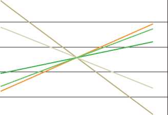
40% 60% 80% 100% 120% 140% 160%
Change in variable
120
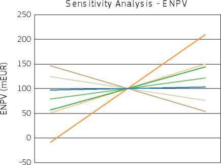
40% 60% 80% 100% 120% 140% 160%
Change in variable
Investment
Fin. O&M costs (excl. reinvestment cost) Demand for services Revenues from leasing of infrastructure Revenues from data transmission services
Econ. Investment cost (incl. reinvestment)
Econ. O&M costs (excl. reinvestments)
Demand for services
Consumer surplus
Business benefits
e-government savings
e-health savings
The high switching values for the critical variable (investment costs) identified in the financial analysis suggest that the project is most likely to maintain a negative FNPV(C), even under reasonably optimistic assumptions on the change in investment costs, thus supporting the project with an EU grant appears justified. The most critical variable for the project's ENPV is the change in demand, which shows a switching value of 46 %. The demand analysis was based on the detailed analysis of market trends and the region's demographics, and was further supported by consultations with network operators, hence the probability of a situation in which the project fails to secure the necessary demand being low. All other variables show notably higher switching values, which means that the result of the economic analysis is robust and the project will remain worthy of EU financing even under pessimistic assumptions.
The risks of the project are evaluated in the following risk matrix. The analysis considers demand side risks and financial risks during implementation and operations, as well as institutional and legal risks. The identified risk factors are evaluated against their probability of occurrence and their expected impact on the project. Finally, risk prevention and mitigation measures are established to manage the risk (see Table 5 for a summary).
Table 5 Project risks
|
Risk description |
Probability* (P) |
Severity* (S) |
Risk level* (= P*S) |
Risk prevention/ mitigation measures |
Residual risk |
|
Demand risk | |||||
|
Low investments in last-mile network by service providers |
B |
IV |
Moderate |
Market consultations with potential last-mile network operators were carried out by the project promoter during preliminary network design. |
Low |
|
Low take-up by end-users from service providers |
C |
V |
High |
Actively promote the project amongst the potential users and local public administration through appropriate publicity campaigns. An appropriate budget for this purpose has therefore been included in the project investment cost. Implement demand stimulation activities, like training and promotional measures by the project promoter. Coordinate with complementary priorities of the OP: subsidy for the end-users with low income, and development of new e-government and e-health services. |
Moderate |
|
Risks during implementation | |||||
|
Change of the project investment costs |
C |
III |
Moderate |
An active dialogue between the project promoter and the private sector was carried out at the stage of project development (to ensure correct cost estimations), which will be continued during the DBOT procurement process (to ensure that the private sector understands the project requirements). The project promoter shall identify and secure other sources of funding in case additional financing is required (i.e. bids for DBOT contract are higher than expected). |
Low |
|
Implementation delays |
C |
V |
High |
The implementation plan takes into account time contingencies. The DBOT contract will further contain detailed clauses in relation to dates when given parts of the network must be delivered or compensatory payments will need to be paid by the private partner. This will allow sharing the implementation risk with the private partner and give an incentive to the private partner to limit delays. Ensure an adequately skilled internal resource is in place on the project promoter’s side for implementation. Assign a full-time project manager on the project promoter’s side and manage project in a structured environment. Actively use dialogue sessions involving all key personnel, including private sector partner, to ensure implementation is on track. |
Moderate |
|
Institutional risks | |||||
|
Unsuccessful ERDF application, lack of EU funding |
A |
V |
Moderate |
The project promoter ensured that there was regular communication with the managing authority and the European Commission at an early stage of project development so as to identify and address any issues in a timely manner. Additional external support was sought to assist in the project development (private consultants, JASPERS). |
Low |
|
Legal risks | |||||
|
Risk description |
Probability* (P) |
Severity* (S) |
Risk level* (= P*S) |
Risk prevention/ mitigation measures |
Residual risk |
|
Procurement delay |
D |
III |
High |
Prepare detailed tendering documentation by experienced internal/external experts appointed by the project promoter. Introduce time contingencies in project planning by the project promoter taking into account possible procurement delays (i.e. management of claims by competitors). |
Moderate |
|
Risk of not obtaining required property rights |
B |
II |
Low |
The project promoter ensured close cooperation with the local administration authorities at the stage of network pre-design. The project promoter took into account the minimum number of permits required when preparing the pre-design of the network. Each year, areas where permits can be problematic need to be identified. Possible alternative locations will be the private partner’s responsibility at the stage of the final network design. |
Low |
|
Financial risks during operations | |||||
|
Increase in project operating costs |
C |
IV |
High |
Regularly verify the project cost assumptions at the stage of network implementation by the private partner. Ensure close dialogue between the private partner and the last-mile infrastructure operators so as to minimise future operating costs at the design stage. Agree on possible modifications of the level of rent between the project promoter and the private partner. Identify sources of funding by the project promoter and private partner to cover any potential increase in operating costs assigned to the project promoter or private partner. |
Moderate |
Evaluation scale: Probability: A. Very unlikely; B. Unlikely; C. About as likely as not; D. Likely; E. Very likely.
Severity: No effect; II. Minor; III. Moderate; IV. Critical; V. Catastrophic.
Risk level: Low; Moderate; High; Unacceptable.
The risk analysis indicates that without appropriate risk prevention and mitigation measures the overall risk level for the project would be unacceptably high. However, the measures put in place to prevent the occurrence of the identified risks and/ or mitigate their adverse impact should lower the individual risk levels and result in an overall manageable and acceptable residual risk for the project. The risk of the project failing to achieve its targeted objectives at a reasonable cost can be considered to be low.
The research, development and innovation (RDI) infrastructure is the generic name for investment projects that are designed and operated according to very different specifications. In some cases their features are unique, and cannot be analysed with the same degree of standardisation of methods as, for example, in railways or in water, for which there are several decades of evaluation experience and a large library of appraisal documents.
Moreover, while the target groups of other infrastructures are relatively well identified, e.g. passengers for high-speed rail or residents in a urban area for solid waste management, the multifaceted nature of RDI is such that many types of direct and indirect target groups are involved, from businesses to the general public. Each of them has standing in the CBA, and this makes the evaluation of infrastructures a particularly complex task. 309
It is expected that over the next planning period, a portfolio of CBAs of RDI infrastructures will be gradually built within the Member States, following the high priority given to research and innovation for the EU growth strategy, and this chapter offers some hints about how to proceed for applicants of EU funds in the context of cohesion policy.310 Differently from the other chapters of the guide, this chapter does not include a complete case study, because of the large variability of types of RDI infrastructures. However, it includes several practical examples.
Cost-benefit analysis of RDI infrastructures is a new field and the project proposer should be aware that, at the same time, it requires a solid understanding of the principles of CBA, professional experience in project evaluation in different areas and a very flexible practical approach tailored to the specific project under appraisal.
Research, development and innovation are at the core of the policy agenda as key drivers of sustainable long-term economic development.311 In the last decade, the European Union has pushed towards the expansion of RDI capacities and the increase of expenditure in RDI activities, with the final objective of making the EU a leading knowledge-based economy, and regaining its place as a world leader in science and technological progress.
Building on the intent of increasing public and private expenditure in research and development throughout the EU Member States so as to approach 3 % of GDP by 2020, the European Commission adopted the Europe 2020 Strategy in 2010, which puts RDI at the top of the EU agenda for smart, sustainable and inclusive growth. In order to take a more strategic and overarching approach to innovation, improve the innovation systems in the EU and overcome fragmentation, the Commission launched the ‘Innovation Union' flagship initiative, aimed to ensure that innovative ideas can be turned into products and services that create economic growth and jobs.312
Efforts to promote RDI throughout the EU Member States may include a variety of initiatives. The European Commission's Guide to Research and Innovation Strategies for Smart Specialisations (RIS3) (2012) identifies a mix of delivery instruments that could be part of a regional innovation strategy, such as cluster development, measures of innovation friendly business environment, research infrastructures, centres of competence and science parks, support to internationalisation, financial engineering instruments and others. Among all these, only operations whose total eligible costs exceeds EUR 50 million and fall within the definition of major projects, according to Article 100 of EU Regulation No 1303/2013, should be appraised through CBA.
RDI infrastructures can be promoted by enterprises and/or universities, research institutes and other entities, often in collaboration with each other. Enterprises include both large businesses and SMEs, which could participate either individually or in aggregation with other enterprises (e.g. clusters, consortia, etc.). The types of eligible investment in RDI and the volume of public aid should comply with the Community framework for State aid.313
Selected policy and regulatory documents relevant to the RDI sector are listed in the box below.
European Commission Communication, ‘Europe 2020. A strategy for smart, sustainable and inclusive growth’,
COM(2010) 2020 final.
European Commission Communication, ‘Europe 2020 Flagship Initiative - Innovation Union’, COM(2010) 546.
European Commission Communication, ‘Regional Policy contributing to smart growth in Europe 2020” - COM(2010) 553.
Commission Staff Working Document, ‘A rationale for action’, SEC(2010)1161 final, accompanying document to COM(2010) 546.
European Commission Communication, ‘A Reinforced European Research Area Partnership for Excellence and Growth’, COM(2012) 392 final.
European Commission Communication, ‘A Stronger European Industry for Growth and Economic Recovery’
COM(2012) 582 final.
European Commission, DG Regional Policy, ‘Guide to Research and Innovation Strategies for Smart Specialisations (RIS3)’, March 2012.
European Commission Green Paper, ‘From Challenges to Opportunities: Towards a Common Strategic Framework for EU Research and Innovation funding’, COM(2011) 58.
European Commission Communication, ‘Framework for State aid for research and development and innovation’,
(2014/C 198/01).
European Commission Communication, ‘Preparing for our future: Developing a common strategy for key enabling technologies in the EU’, COM(2009) 512 final.
European Strategy Forum on Research Infrastructures - ESFRI ‘Research infrastructures and the Europe 2020 Strategy’. Innovation: How to convert Research into Commercial Success Story?, Study of the European Commission, 2013
The innovation process is generally associated with a number of activities, related to fundamental research, applied research, experimentations and technological development, production and commercialisation. When RDI investments are characterised by a clear prevalence of one type of activity over another, it is possible to distinguish RDI projects as investments focused either on research and development, or on innovation.
In what follows, the following definitions are adopted.
• Research and development infrastructures are science-related physical realisations (laboratories, facilities, etc.) developed with the main purpose of acquiring new knowledge in a given scientific and technological field.
• Research and development infrastructures, in turn, can be discriminated between:
- infrastructures for fundamental research, i.e. infrastructures that are meant to undertake theoretical or experimental work primarily to acquire new knowledge on the underlying foundations of phenomena and observable facts, without any direct practical application or use in view; and
- infrastructures for applied research and experimental development, i.e. infrastructures directed to a more practical purpose, where research and investigation are aimed at the acquisition of new knowledge and skills for developing new products, processes or services or for bringing about a significant improvement in existing products, processes or services, which are not yet directly intended for commercial use.
• Innovation infrastructures are infrastructures aimed at combining knowledge and technology for the development of new or improved products, services and business processes that could be sold on the marketplace.
In many cases, however, it is not possible to sharply distinguish between research and development infrastructures and innovation infrastructures. RDI infrastructure projects in reality are likely to encompass multiple activities, ranging throughout the whole innovation process spectrum (section 7.4 contains some examples of typical RDI projects). The combination of knowledge creation with knowledge transfer activities, ultimately intended for the commercialisation of research results, aims to produce direct economic impact on the regional/national dimensions in terms of industrial competitiveness.314
According to the new European strategic orientations, defined in the Europe 2020 strategy, and in line with thematic objective 1 ‘Strengthening research, technological development and innovation' of the EU Regulation No 1303/2013 (Article 9), during the 2014-2020 programming period the European Commission will focus on reinforcing links between education, business, research and innovation. Accordingly, major projects are expected to target, in particular, innovation and applied research and technological development infrastructures, which are closer to the market, as a means of translating knowledge into tangible and immediate business opportunities.
The ERDF could only support investments in building fundamental research in exceptional cases, insofar as they are expected to produce tangible effects for regional and national economies and create a competitive environment in which the endogenous strengths of given regions (reflected in specific existing or emerging industries) are translated into market innovations.315
The analysis of the socioeconomic context is crucial to the development of RDI infrastructure as it affects the decision on size, sector and purpose of the infrastructure. The degree to which the RDI infrastructure to be developed fits into the (regional, national and international) context and are tailored to the RDI needs should be clearly assessed.
The analysis of the socioeconomic trend provides important information for the assessment of existing research and innovation gaps and needs, and should therefore be the starting point for the project appraisal. Information related to the socioeconomic trend should also be discussed in detail because they are likely to influence the forecasting of benefits (see section 7.8).
From the perspective of policy and legislative context elements, investments in RDI should fit into the smart specialisation strategy of a country or region and thus contribute to its place-based economic transformation, supporting territorial competitive advantages and potentials. Reference to other relevant policy and programming documents should be made explicit.
An analysis of the industry in the region/area that can benefit from the RDI project is needed for the assessment of needs and the verification of the project's relevance, especially when the scope is to trigger innovation processes. Conditions and the capacity for existing research facilities, human capital endowment (in terms of students and researchers) and employment opportunities should be carefully assessed to identify the bottlenecks that the project is aimed to fix. The potential of cost savings, efficiency gains and economies of scale achieved through collaboration with other countries/regions and possibly existing infrastructures should be explored.
The main context information that is generally relevant to RDI infrastructures and which should be discussed in the project appraisal, where applicable, is shown in Table 7.1. Possible data sources include Eurostat, the OECD, the European Spatial Planning Observation Network (ESPON), Innovation Union Scoreboard indicators, etc.
Table 7.1 Presentation of the context: RDI sector
|
Information | |
|
Socioeconomic trend |
- National and regional GDP growth - Magnitude and characteristics of industry in the catchment area of the infrastructure - Demographic statistics (population size and growth) - Education statistics (current and future student body, percentage of population having completed tertiary education, etc.) - Percentage of population employed in the education sectors - Gross domestic expenditure in research and development (in absolute terms, as a share of GDP, per capita expenditure) - Degree of achievement of national targets related to the RDI sector - Education background: number of graduates, students, educational specialisation |
|
Policy and legislative framework |
- Reference to EU sector policy documents (see above) and other horizontal policies - Reference to the priority axis and the interventions areas of the OP - Reference to the Regional and Innovation Strategy for Smart Specialisation (RIS3) - Reference to national and regional strategic documents and development plans - Connection with other EU programmes and initiatives - Reference to State aid legislation |
|
Geographical conditions and availability of resources |
- Geographical proximity to universities, industries and other research laboratories to favour networking and collaboration - Geographical proximity to the research object (e.g. as regards facilities for studying a particular biological habitat) - Proximity to ancillary services or facilities (e.g. housing and accommodation) - Accessibility - Number and specialisation of scientists and students in the infrastructure’s reference area and field - Availability of well-established technical engineering expertise in the infrastructure’s reference area |
|
Current level of research and innovation |
- Percentage of employees in the research and development sector - Knowledge intensity of businesses in the region - Number of patent applications and patent per capita in different economic sectors - Scientific publications among the top 10 % most cited publications worldwide as a percentage of the total scientific publication of the country - Venture capital investment as a percentage of GDP - SMEs innovating in-house as a percentage of SMEs - SMEs introducing product or process innovations as a percentage of SMEs - Sale of new-to-market and new-to-business innovations as a percentage of turnover |
|
Conditions of the existing research facilities and infrastructural needs |
- Current state of the existing infrastructures and facilities in the same scientific/technological field - Current number of research centres in the same field in the infrastructure’s reference area and in other regions/countries - Benchmarking with other RDI infrastructures operating in the same field in other regions/countries, e.g. in terms of availability of spaces and experimental areas in existing laboratories, scientific and technical characteristics of existing installations and equipment, etc. - Past and present scientific activity carried out by the project promoter, e.g. in terms of research budget breakdown, number and value of research projects conducted, publications, awards, scheduled directions of research - Cooperation agreements with existing entities or other relevant research programmes |
Source: Authors
RDI projects can be associated with a multitude of long-term objectives, including amongst others:316
• contribute to the advancement of knowledge and maintaining Europe at a world-class level in science and technology;
• accelerate the development and deployment of innovative, enhanced, more efficient and higher value added products, processes or services that meet the demand of customers and users;
• strengthen the cooperation between research, innovation, education and business to create more jobs and increase economic competitiveness;
• enhance the attractiveness of a cluster or science park for investors and companies;
• increase the number of graduates in specific fields to foster smart specialisation;
• help address societal challenges in a number of fields, including, for example, energy security, sustainable transport, climate change and resource efficiency, health and ageing, environmentally friendly production methods and land management, etc.;
• develop and strengthen the European Research Area by making national research systems more effective, ensuring optimal transnational cooperation and competition among researchers, and guaranteeing access and transfer of knowledge;
• reduce the ‘permanent' brain drain in certain geographical areas and/or scientific fields by promoting the development of RDI infrastructures, which could persuade scientists and students not to move elsewhere;
• promote the mobility of researchers and associated exchange of ideas;
• increase technological spillovers potentially generated from large-scale RDI infrastructures;
• stimulate students to take up scientific studies and undertake a career in a specific scientific field.
When defining the project objectives, the promoter shall always state how the project will help contribute to specific national
and EU policies, e.g. Horizon 2020, Smart Specialisation Strategy, as well as the objectives of the relevant OP and priority
axis.
The proposed project must be described in detail as a self-sufficient unit of analysis.
When RDI investments consist of single-site facilities, i.e. a single or a set of infrastructure and equipment located in a single physical location, as defined by ESFRI (2012), the project identification becomes relatively straightforward. As an example, single-site RDI infrastructures include telescopes, medical research facilities, laboratories for technological experimentation and others.
Geographically distributed RDI facilities, consisting of a network of infrastructures and equipment located in different places (or even different countries), can also be identified as a self-sufficient project if there is a strong functional relationship among all of its parts, meaning that the distributed facilities cannot operate and/or produce RDI results without contributions from any of the facilities. Examples of the distributed RDI infrastructures could be research centres in the field of climate change, biosciences, geology, and with measurement stations or systems of satellites located at different sites.
RDI investments aimed at fostering cooperation between a number of research facilities and knowledge transfer/innovation facilities, which are located in the same area (e.g. city or region) but are not incorporated within one single-site infrastructure
stricto sensu, could still be considered as a single project and a self-sufficient unit of analysis for the purpose of the CBA, as long as they create strong synergies, critical mass and achieve cost savings for each facility involved. Project boundaries need to be precisely traced and the rationale for conceiving separate infrastructures as a unitary major project should by justified.
In any case, the proposed project should clearly aim at addressing a relatively well-defined research or innovation objective. Investments merely focusing on the construction or purchase of new university buildings not directly intended for research purposes, or an improvement in the energy efficiency of research facilities should not be considered as RDI projects.
An indicative and far from exhaustive list of typical major RDI projects that are expected to be financed by the ERDF are presented in the table below. For illustrative purposes, they are distinguished between infrastructures mainly for (applied) research and development, those mainly for innovation and those for both research/development and innovation, depending on the possibility of identifying the prevalent activity carried out.
Table 7.2 Examples of typical RDI infrastructural major projects
|
Type of RDI infrastructure |
Examples of major projects and activities/services offered |
|
(Applied) research and development infrastructures |
- Competence centres and laboratories and equipment specialised in a specific technology or field (e.g. clinical research centre, microscopy facilities, laser light facilities, laboratories for biological studies, etc.) - R&D centres and laboratories for research organisations (universities, research institutes, other bodies) - Facilities and/or equipment for developing and/or testing prototypes and innovation, not yet intended for commercialisation (e.g. large-scale demonstrator to test innovation in a real-life environment) |
|
Innovation infrastructures |
- Laboratories and equipment for single private enterprises to support the development, testing and manufacturing of innovative products or services (e.g. pilot plants) - Technology park including facilities for innovation: business incubators, innovation centres, centres for experimental development, living labs, fab labs, Design Factory, spin-offs, etc. |
|
Infrastructures for research, development and innovation |
- Science and technology parks, comprising applied research laboratories and innovation facilities (business incubators, innovation centres, centres for experimental development, living labs, fab labs, Design Factory, spin-offs, etc.) - Laboratories and equipment for aggregations of private enterprises, research institutes, and universities, to support the development, testing and manufacturing of innovative products or services - Research centres with applications of research outputs to final users (e.g. clinical research infrastructures developing new health protocols for the treatment of patients at the centre) |
As presented in Chapter 2, the demand analysis implies identifying the need for an investment, which is expressed by the current and future demand. Quantifications of the demand in the scenarios with and without the project are both essential for formulating the project demand projections in incremental terms. The demand analysis should be carried out before the option, financial and economic analyses, since it provides inputs that are necessary for the subsequent appraisal steps.
Different to other sectors, which are more focused on the delivery of a limited set of specific services, the RDI sector has a particularly heterogeneous variety of possible projects, to which any number of diverse drivers of demand can be associated. The demand of RDI infrastructures is actually driven by the social and economic needs expressed by a multiplicity of target groups, i.e. stakeholders who/which will ultimately benefit from the intervention. These may include both project users and non-users, whose welfare will be affected by the construction, operation and services provided by the infrastructure. Such multiplicity prevents any generic discussion about the demand analysis, which should be based on the project specificities.
To simplify this, three macro categories of target groups, which drive the demand for the RDI project at regional and/or national level, can be identified:
• businesses, including SMEs and large enterprises, high-tech businesses, spin-offs and start-ups, which enjoy the services provided by the project and/or the indirect spillover effects;
• researchers, young professionals and students, who would use the RDI facility to carry out their own research to increase scientific and technological knowledge in a given field, or for a training programme;
• target population and the general public, who are attracted by the project outreach activities or who are the direct or indirect target of research.
In principle, the list may be broken down to a more detailed level of analysis (see below).
It is important to understand that not all categories of target groups may be involved in the same project. In fact there is no rigid correlation between the taxonomy of RDI infrastructures introduced in previous sections of this chapter (section 7.1 and 7.4) and the target group(s). Some categories of actors but not others could potentially be involved in fundamental or applied research, development and innovation infrastructures, depending on the specific project features. For example, hi-tech businesses may be important as recipient, albeit indirect, of a fundamental research project, while they may not immediately be involved as users in applied research.
For each identified target group, the project promoter has to examine those specific factors that could influence the volume and trend of demand. Different methods can be used for demand projections, as suggested in Table 7.3.
The project promoter should pay particular attention in dealing with uncertainty when forecasting future demand from the potential target groups. Optimism bias in the identification and quantification of the demand should be avoided and the risk attached to demand projections should be tested in the risk assessment phase (section 7.9). Some hints on how to forecast future demand are provided in section 7.8, with specific reference to the valuation of economic benefits.
Table 7.3 Data, methods and outputs of the demand analysis
|
Target group |
Examples of factors driving the demand |
Possible methods for data gathering and estimation |
Examples of output from the demand analysis |
|
Businesses |
- Average growth of the industrial base in the RDI project field in the last years - Average annual profitability of the industrial base in the RDI project field - Knowledge intensity of businesses in sectors related to the RDI project - Access to venture capital funds possibly stimulating the establishment of start-ups - Level of public investment in fields related to the RDI project - Capacity of the incubator or other RDI facilities - Number of enterprises potentially interested in using the services provided by the RDI project - Level of involvement of enterprises in the governance of the infrastructure |
- Statistical analysis of historical data - Databases of financial information and other details about companies - Track record of the business in producing patents and innovation in general - Relevant literature and existing studies - Benchmarks with similar RDI projects - Interviews, surveys, consultations - Letters of intent for potential industrial research collaborators - Details for potential collaborative research projects - Smart specialisation priorities and allocation of budget resources in the related fields |
- Annual number of spin-offs /start-ups expected to be generated/supported by the project - Expected number of businesses using the infrastructure to develop new/improved products and processes - Expected annual number of patents registered by project users - Expected trend of revenues from licensing and technology transfer - Expected number of non-user businesses possibly enjoying knowledge/technology spillovers |
|
Researchers, young professionals and students |
- Number of scientists operating in the RDI project field and in the geographical area targeted by the infrastructure - Number of existing facilities operating in the same field and competing with the RDI infrastructure - Technical characteristics and scientific potential of the RDI infrastructure - Reputation and track-record of researchers - RDI project capacity to attract funding and users - Current number of students in the RDI project field or related fields in the geographical area targeted by the infrastructure - Applicability of RDI skills acquired from the research project in the labour market - Potential for generating income through student fees and private sponsoring |
- Statistical analysis of historical data - Relevant literature and existing studies - Benchmarking with other similar, existing RDI facilities - Scientometric analysis of publications and citations in the RDI project field - Demographic projections - Surveys, interviews, consultations to assess the attractiveness of the RDI sector among students - Unemployment rates of graduates / speed to find employment after graduation - Number of business scholarships sponsoring students’ fees |
- Annual number of researchers who will directly use the RDI infrastructure - Number of scientific publications expected to be produced by the project users - Number of citations expected to be received by users’ publications - Annual number of young professionals and students who will use the RDI infrastructure - Duration of the training programme at the RDI infrastructure - Revenues from student fees |
|
Target population and general public |
- Number of people affected by environmental and health risks and virtually targeted by the RDI project - Existence of knowledge transfer agreements to other RDI infrastructures - Attractiveness and appeal of the RDI infrastructure among the wider public - Provision of outreach activities by the project promoter - Price charged for guided tours or other outreach activities |
- Statistical analysis of historical data - Relevant literature and existing studies - Benchmarks with similar RDI projects - Interviews, surveys, consultations |
- Annual number of people potentially targeted by the project - Annual number of patients treated by innovative medical technologies - Annual number of people potentially interested in visiting the project or potentially targeted by other outreach activities |
KJ
\l
cn
GUIDE TO COST-BENEFIT ANALYSIS OF INVESTMENT PROJECTS
The project that is proposed for implementation should be justified among a number of alternative options. The option analysis aims at identifying the most promising project option that can achieve the expected objective given a certain demand.
The baseline for the option analysis is the description of a scenario without-the-project for which alternative options can be conjectured. It is important to bear in mind that all possible options should be defined as alternative ways to achieve the same specific project objective, for example in terms of performance improvement of products and process, an increase in research capacity, or local development in the framework of a smart specialisation and place-based strategy. Projects aiming at different objectives cannot be compared across each other.
RDI project options could differ one from another from multiple perspectives. When deciding to build, for instance, a new competence centre, the project promoter faces a number of choices concerning the project localisation in a given region or country, the technological solution employed for carrying out experiments, and many other factors. A set of possible options can thus be described for each particular aspect of the project (see the box below for some examples).
Listed below are some examples of alternative options that are likely to be presented in the option analysis of RDI
projects.
- Strategic options: A set of alternatives (e.g. A, B, C, D) which may concern the structure of the overall project. For example, alternative A may involve the regrouping of different research centres, while B proposes the construction of a new research facility.
- Technological options: A set of alternatives (e.g. A, B, C, D), which may concern different technologies to be purchased by the project. Several (more or less sophisticated and cost-intensive) technological set-ups may be available on the market, which allow carrying out the proposed research.
- Location options: A set of alternatives (e.g. A, B, C, D) which may concern the location or the geographical set-up of the project. For example, a higher education and research infrastructure project may be located in one of several locations, or split between a number of different locations. In other cases, the choice could be about whether to build the RDI facility in one city or in another, or in the urban centre rather than in the suburbs or countryside.
- Architectural options: A set of alternatives (e.g. A, B, C, D) that concern the architectural design of the building where a project is located. For example, a research centre may be located in a newly built building or in an old refurbished building.
Source: Adapted from JASPERS (2013)
Each option should be assessed against a number of criteria, such as:
• its expected costs,
• expected revenues,
• expected economic benefits, including positive and negative externalities,
• possible wider regional effects,
• implementation time,
• degree of uncertainty and the risk involved.
Options should be compared across each other by means of both a multiple criteria analysis and a simplified CBA, where rough estimates of financial and economic flows are used to calculate financial and economic performance indicators. See Chapter 2 for details. The proposed project should be the one that combines the best performing alternative options within each range of available options, in such a way that it allows the greatest benefits to be achieved in the most efficient way.
When a similar economic impact is expected to be achieved using different options, the preferred option can be selected by considering either the financial net present value (the lower the financial net present value the more efficient the project is) or other qualitative aspects arising from the multi-criteria analysis.
Categories of financial costs, which are generally related to RDI infrastructures, are synthetically presented in Table 7.4 below.
Table 7.4 Typical investment, operation and maintenance costs of RDI infrastructures
|
Investment cost |
O&M costs |
|
- Planning and design costs |
- Materials and equipment |
|
- Land acquisition |
- Consulting services |
|
- Construction costs, possibly disaggregated by civil works and |
- Cost of scientific personnel |
|
installations, materials, labour, etc. |
- Cost of administrative and technical staff |
|
- Energy, waste disposal and other utilities consumed during |
- Cost of obtaining and maintaining patents |
|
the construction period |
- Energy, waste disposal and other utilities |
|
- Road access |
- Promotional campaigns and other outreach expenditure |
|
- RDI equipment, including information technologies |
targeted to the general public |
|
(particularly for data storage or elaboration) |
- Training courses connected to the infrastructure’s |
|
- Intellectual property purchase costs |
operation and management |
|
- Testing |
- Removal of potential pollutions / brownfield site |
|
- Start-up costs |
treatment at the end of the life cycle of the infrastructure |
Source: Authors
Cost savings in O&M or investment achieved through the project's implementation should also be accounted for and included on the cost side of the analysis, as a negative, i.e. as decreasing costs in respect of the counterfactual situation.
The project promoter may not pay for goods, services and staff for the construction or operation of the project; external parties may provide these in-kind. This is not unusual for investment projects promoted by public research bodies and universities. In-kind contributions should be treated as follows:
- in the financial analysis, in-kind contributions are not to be included among the project’s costs because they do not represent an actual cash flow for the project promoter;
- the corresponding economic value of in-kind contributions should be included on the cost side of the economic analysis, where all project-related costs for society have to be considered;
- the residual value of in-kind material and equipment provisions should be considered in both the financial and economic analyses.
RDI infrastructure projects can gain revenues from the provision of a variety of services to public and private users. Services provided and revenues attained may vary greatly from one project to another. Table 7.5 below shows a (non-exhaustive) list of typical inflows that shall be considered as operating revenues.
As compared to other types of projects, RDI facilities are more often than not largely dependent on public financing sources and these financing sources can be very diversified. Besides the national/regional capital contributions that are common to all projects, there could be a variety of other contributions to the research project, granted by European, national or regional public and private parties. Such financing mechanisms may vary widely across countries in their characteristics depending on the country-specific institutional set-ups.
The project promoter should carefully assess whether a financial inflow, particularly if granted by a public institution or agency, should be considered as either a source of financing or operating revenues. In general, research contracts or contributions granted from the public sector, either through competitive or non-competitive arrangements, should be considered operating revenues (and therefore included in the financial profitability analysis and in the calculation of the discounted net revenue, in line with Article 61 of Regulation 1303/2013) but only if they are payments against a service directly rendered by the project promoter. This condition is often verified when the ownership of the expected research output is transferred to the contracting public entity and does not remain with the research institution. For example, a grant awarded by a regional public agency to a public research body, directed to the development of a new software usable in the regional hospitals, or a new type of railway signalling system to be installed on the regional railway lines, can be considered a fully-fledged operating revenue for the research project.
Instead, public research funding schemes aimed at covering (part of) the operating cost born by the project promoter, but without involving a transfer of the research output's ownership, shall be considered as sources of financing, but not operating revenues. Following the regulatory provisions317 and in line with the general CBA methodology put forward in section 2.8.4 of this guide, these financing sources shall be considered as ‘transfers from state or regional budgets'. As such, they shall not be included as revenues for the calculation of both the financial performance indicators and the determination of the Union assistance. However, they account for the verification of the financial sustainability. Examples of this category of financing sources include grants from European or national research funding frameworks (such as Horizon 2020), regular or exceptional donations from the State, contributions by the National Health Service to university hospitals, etc.
The degree of uncertainty attached to the acquisition of special public research funding, meant either as operating revenues or sources of financing, over the project's lifetime is often very high and this could significantly affect the project' sustainability and profitability indicators. In this regard, the project promoter should avoid excessive optimism bias. The uncertainty attached to project inflows should be duly discussed and analysed, even by means of the risk assessment set of procedures.
Table 7.5 Typical revenues and sources of financing of RDI infrastructures
|
Examples of operating revenues |
Examples of financing sources |
|
- Licence revenues gained from patents’ commercialisation |
- National/regional public contributions |
|
- Sale of consultancy services |
- National/regional private contributions |
|
- Revenues from industrial research contracts and pre-commercial |
- EU contribution |
|
procurement contracts |
- Other national/regional funding schemes for RDI |
|
- Entry fees to the laboratory and for the use of research equipment |
activities |
|
charged to researchers and businesses |
- Public grants to research, e.g. under the Horizon |
|
- Student/master/PhD fees |
2020 framework |
|
- Spin-off equity realisations - Research grants involving a transfer of ownership of a specific research output - Sale or rent of new buildings used for the project’s objective - Revenues from the target population using the research outputs (e.g. patients receiving an innovative treatment) - Revenues from outreach activities to the wider public (e.g. bookshops’ sales, entry fees, etc.) |
- Ordinary public transfers |
Source: Authors
The main difficulty, which has often discouraged the use of a proper CBA in the context of RDI infrastructures, is the estimation of the social benefits from a range of diverse projects, which may span from research centres on climate change to scientific and technological parks, or from high-energy physics research infrastructures to bio-molecular research facilities. Some guidance is offered below about the practical estimation of social benefits. The perspective, as for the rest of the guide, is ex ante, when uncertainty about the benefits of the RDI infrastructure is greatest.318
The presentation of the economic analysis is structured as follows. Having identified in the previous sections the activities and services generally delivered by RDI infrastructures, as well as the main categories of (user and non-user) stakeholders or target groups, a list of typical benefits can be pointed out for each target group (section 7.8.2). For every benefit, in turn, possible approaches for forecasting the quantities of benefit output over the project's time horizon and giving them an economic value are examined. Then, section 7.8.6 briefly deals with the special angle of impact on regional development and competitiveness, and section 7.8.7 shows possible future methodological development in the context of fundamental research projects.
In order to value the social benefits of any project, as a first step the project proposer needs to understand who is going to be targeted, either directly or indirectly, by the services provided by the infrastructure. Typologies of actors targeted by the project should have already been identified for the purpose of the demand analysis (see section 7.5). As a next step, the following questions need to be addressed:
• how is the benefit for each target group defined and how can it be measured in quantity terms?
• how can the quantities of benefits be predicted over the time horizon of the project?
• how is the marginal social value of the benefit estimated?
The total economic value of the expected benefits is then obtained as a benefit quantity times their marginal social value. These basic notions of CBA are repeated here because they should be firmly and consistently applied in the domain of RDI infrastructure, without being discouraged by the special, various and challenging nature of their design and operation.
In what follows, typical benefits enjoyed by the three main categories of target groups related to RDI projects and already listed in section 7.5 (businesses; researchers, young professionals and students; target population and general public) are discussed. For the sake of clarity, it is useful to break down the list of broad categories of target groups into more specific items.
Benefits for businesses319
This category of target group is particularly heterogeneous and could potentially include a large variety of actors, either users or non-users of services offered by the project. A possible list of targeted businesses is provided below.
• New businesses, i.e. technological start-ups and spin-offs established via the project implementation and/or those enjoying the services provided by the incubators and similar infrastructures: these businesses could experience different kinds of benefits, such as decreased business mortality, avoided cost due to the services provided by the RDI facilities, and the development of new or improved products and processes.
• Already existing businesses, which can include the following:
- Large businesses involved in applied research infrastructures, or competence centres shared with universities, other businesses and third parties: the potential benefits for large businesses are the development of new products and processes, in some cases leading to patents or other forms of protection of intellectual property.
- SMEs benefiting from activities and services offered by technological parks and other collective infrastructures supporting R&D: potential benefits could be knowledge spillovers and support to the development of new or improved products and processes. Inventions by SMEs more often than not come from the adaptation of existing knowledge to new fields, and they are not always protected through patents.
- Any other business, either SME or larger, either high-tech or not, which is able to avoid some costs or increase sales because of the impact of new knowledge, spilling over from the research infrastructure as a positive externality. This category comprises, among others, high-tech businesses in the supply chain of the RDI infrastructure, contributing to the development of innovative equipment, materials and software, and benefiting from learning-by-doing effects.
Benefits for researchers, young professionals and students
• Academics and researchers involved in the design, operation and use of experimental machines of fundamental and applied research facilities, and other academics benefiting from the new scientific literature created: the potential benefit enjoyed by academic researchers are publications and citations in scholarly journals; less frequently the benefit could take the form of registration of patents or other forms of intellectual property protection.
• Young researchers within businesses or outside academia: an increase of human capital benefit can be ascribed to this category of actors, particularly when young professionals, post-doctoral researchers and early career researchers are involved; the increase of social capital through networking with peers and established researchers can be another possible benefit.
• Students, usually at graduate level, for example involved in training or the preparation of their doctorate (PhD) dissertation with fieldwork at the research infrastructure, less frequently at the technological development and innovation infrastructure. As with young researchers, students could enjoy the human capital and social capital development effects.
Benefits for the target population and general public
• Population in areas of environmental risk: Due to the new research or surveillance methods developed in the RDI infrastructures, the population could benefit from the costs avoided and lives saved in relation to major risks, such as the effects of climate change, earthquakes, floods, fires, pollution, etc.
• Population at health risk: This category includes patients associated with medical or pharmacological research infrastructures in the field of new therapies, or other members of the public targeted by the RDI project who experience health benefits in terms of avoided mortality and increased quality of life. Other patients (non-users of the research infrastructure) may also benefit from knowledge spillovers to other contexts.
• General public interested in science and technology arising from onsite visits to the infrastructure, virtual visits to the project's websites and social networks, availability of educational publications and information in the media as part of the outreach activities of the team managing the RDI infrastructures. The related use-benefit is in terms of cultural effects, valued through the marginal willingness-to-pay for this form of cultural activity.
Browsing the above-mentioned types of benefits (listed in the Table below),320 it can be observed that some of them recur for different types of target groups. For instance, the value of patents as a potential benefit may accrue to large businesses, SMEs, academic scientists or inventors outside academia. Also, it should be borne in mind that the intensity of each benefit may be highly variable across the different typologies of RDI infrastructures. For example, the social benefit of human capital change is highly relevant for applied research infrastructures, where students are often involved in research activities, but is less relevant for technological development and innovation infrastructures. However, many projects may combine some ingredients of the main types of RDI infrastructures (i.e. infrastructures for research, technological development or innovation), and only a case-by-case appraisal can tell which category of benefit is more or less important for a specific project.
Table 7.6 Target groups, benefits and related evaluation approach: an illustrative synopsis
|
Benefit |
Evaluation approach |
Target groups | |||||||
|
Businesses |
Researchers, young professionals and students |
Target population and general public | |||||||
|
Already existing business es |
Spinoffs and startups |
Academics and researchers |
Researchers within businesses or outside academia |
Stu dents |
Target population at environmental risk |
Target population at health risk |
Gen eral public | ||
|
Establishment of more numerous or more long-lived start-ups and spin-offs |
Shadow profit |
+ + |
+ |
+ |
+ | ||||
|
Development of new/improved products and processes |
Shadow profit or value of patents |
+ + |
+ + |
+ |
+ | ||||
|
Knowledge spillovers to non-user businesses |
Shadow profit or avoided cost |
+ + |
+ | ||||||
|
Value of scientific publications |
Marginal production cost |
+ + |
+ | ||||||
|
Human capital development |
Incremental lifelong salary |
+ + |
+ + | ||||||
|
Social capital development |
Qualitative analysis |
+ |
+ + |
+ + | |||||
|
Reduction of environmental risk |
Avoided cost or WTP |
+ |
+ + | ||||||
|
Reduction of health risk |
VOSL or QALY |
+ + | |||||||
|
Cultural effects |
WTP |
+ + | |||||||
Note: ++ very relevant; + moderately relevant; VOSL: value of statistical life; QALY: quality-adjusted life year Source: Authors
Businesses can experience a variety of benefits, depending on their relationship with the RDI project. Benefits can be in the form of the establishment of spin-offs and start-ups, the development of new or improved product and processes (possibly, but not necessarily, leading to patents), the provision of special services to user-businesses and knowledge spillovers to non-user businesses.
Whatever the benefit experienced by businesses is, the general rule is that any change beneficial to a business should be valued by incremental shadow profits, as compared to the without-the-project situation. This is in line with the CBA concepts and methodology described in Chapter 2. For the sake of simplicity, in what follows, the notion of ‘profit' (instead of ‘shadow profit') is used, with the understanding that market distortions should be taken duly into account. For example, if targeted businesses are located in areas characterised by high unemployment, the shadow profit will be higher than the gross financial profit321 because the shadow wage will be lower than the market wage.
Forecasting expected profits may not be an easy task, mainly because of the confidentiality of information. There are, however, different possible approaches to predict changes in a business's profits, which the project proposer could consider.
For example, for most large businesses or certain categories of business (e.g. for pharmaceutical research companies or enterprises in other specific NACE322 sectors) information about profitability, average costs and sales is available. Databases in the public domain or granted by data providers offer valuable information in this respect. Other useful information is anticipated from the European Commission's ongoing study of the average profitability and performance of selected economic sectors.323 Also, in some cases, some disclosure is possible, particularly when compliance with the EU State aid needs to be proven. Benchmarking with similar RDI infrastructures in other contexts could also offer some input to forecast future profits.
Direct estimation of effects of a RDI infrastructure on future profits of SMEs could be even more complex, as official data for micro and small enterprises are usually limited. However, interviews or comparisons with other similar experiences can help to make a conjecture of possible changes in the profitability of businesses, to be tested by the appropriate risk analysis, as discussed later.
Some more detail about estimating the typical benefits of RDI projects for businesses are presented. Given the very specific nature of each RDI project, additional benefits, which do not precisely fit into the list here indicated, may still exist. However, the evaluation methodology is not expected to be significantly different: in general, the benefit to businesses can always be valued through incremental shadow profit. When more relevant or practical, the avoided cost approach could also be applied, as explained below.
Establishment of spin-offs and start-ups
Spin-offs and start-ups are companies engaged in activities with a strong high-tech and innovative business component. While a spin-off is born from the split of an already existing entity into two or more separate units, a start-up is a new entity created from the influence of an existing company or research organisation (e.g. a university). For the purpose of the CBA, the creation of spin-offs and start-ups are considered under the same typology of benefit, since the methodology of valuation is very similar. The mission of spin-offs and start-ups is to develop and bring to the market new products or services that originate from an initial knowledge input transferred from the parent company or organisation. The establishment of spin-offs and start-ups can be one of the intended objectives of innovation infrastructures, as in the case of incubator centres, but is can also be a side effect of fundamental and applied research infrastructures.
The economic benefit arising from the creation of new business units has often been valued, in past project appraisals, by looking at the economic value of the jobs created. However, this approach is not consistent with the CBA theoretical foundations. The economic value of spin-offs and start-ups should be valued as the expected shadow profit gained by the business during its lifetime, as compared to the counterfactual situation. In order not to commit double counting, the spin-off equity realisations and the operating revenues from the sale of consultancy services leading to the establishment of spin-offs and start-ups, which are included in the financial analysis, should not be considered in the economic analysis.
If the RDI infrastructure contributes towards increasing the survival rate of start-ups, the benefit is valued as the expected profit attained by newly created businesses, which survive longer than businesses in the baseline scenario (see a worked example in the box below). Whenever it is reasonable to believe that the main contribution of the RDI project would not be to increase the survival rate of start-ups, but to increase the absolute number of start-ups in the region, then the total expected profit gained by all newly created businesses during their expected lifetime should be included in the analysis. The latter situation can be expected to occur in some circumstances and typically in particularly deprived areas.
An ex ante estimate of the profit of spin-offs and start-ups should be based on the following:
• the annual and total number of spin-offs/start-ups expected to be generated by the RDI infrastructure;
• the expected value of annual profits earned by spin-offs/start-ups in the considered country and sector;
• the average lifetime of spin-offs/start-ups in the considered country and sector.
Such variables can be inferred from official statistics (at regional, national or, where not available, European level) or relevant literature. As far as possible, sector specificities should be taken into account. Official data about similar RDI infrastructures and their own spin-offs/start-ups, located in the same or other regions and countries, could be taken as reference where available.
The benefit for the establishment of any new business should be estimated for the overall expected lifetime of such a business. It is thus very likely that some benefits would continue after the last year of the RDI project's time horizon. The project promoter should make sure that the residual value of the benefit, properly discounted at the social discount rate, is imputed in the last year of the CBA time horizon.
This box presents an example of the valuation of the benefit related to the creation of start-ups. All figures and assumptions hereby reported have a purely illustrative purpose and should therefore not be taken as reference values. The project proposer is invited to rely on project-specific assumptions and sources, and to duly justify the choice of any input value.
In this example, a technological park, provided with an incubator centre for high-tech start-ups, is expected to support 100 enterprises during its time horizon. It is assumed that the average profit of the assisted companies for the first three years will be zero; it then increases to EUR 0.5 million per year (including taxes, interests and the correction for the shadow wage). The social benefit is the difference between the baseline estimate of the profits of the enterprises supported by the project and the counterfactual situation, where a higher mortality rate of businesses is considered. Thus the profit on the additional surviving businesses should only be computed.
The literature and available studies can give indications about the survival rate of start-ups in specific countries and sectors. The graph below shows some illustrative examples. For example, according to Eurostat business demography statistics (Eurostat, 2009), 50 % of all enterprises started in 2001 survived to 2006. According to the Innovation Union Competitiveness Report 2011 (European Commission, 2011), the survival rate of business enterprises established in EU countries in 2003 was between 50 % and 85 % after five years, depending on the country. The European Investment Bank (EIB) (2013) assumes a probability/success rate of 50 % for the average newly created businesses over 15 years.
Examples of start-ups survival rate curves
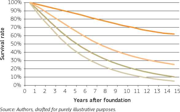
In the considered worked example, the standard survival curve for high-tech businesses in the region where the RDI infrastructure is going to be located indicates that, on average, 30 % of newly established businesses survive after ten years. Based on the evidence from other similar RDI facilities, the project promoter expects that 50 % of newly born businesses, which will receive support by the RDI facility, will close within ten years: in other terms, the support services provided by the project are expected to help reduce a business’s death rate. At year 10, there will be 50 surviving businesses in the incubator against 30 on average in the region. Thus the net effect is 20 more surviving businesses that will still be in operation ten years after their establishment.
The present value of the expected stream of profit for these additional 20 businesses must be computed as a project benefit. It is clear that the benefit value would be highly sensitive to the expected profitability and the survival rates of businesses assisted in the incubator. The appropriate risk analysis shall be implemented to test the impact of these critical variables.
Development of new/improved products and processes
When the RDI infrastructure can be associated with the development of new or improved marketable goods, the changes in shadow profit expected from the sale of such goods should provide the estimate for the benefit. The general remarks made above still apply.
When patents are registered at national, European or other patent offices, the benefit can be estimated by the economic value of patents, provided that double counting with the change of expected profit from the sale of RDI outputs is avoided. In fact the expected value of a patent, in principle, already incorporates the ‘difference between the discounted stream of (shadow) profits since the grant of the patent when the inventor holds the patent, and the equivalent discount stream of (shadow) profits without the patent' (European Commission, 2006: 4).
Attention should also be paid to not including in the economic analysis the financial revenues coming from licences, revenues from research contracts and grants, and entry fees paid by user companies ultimately aimed at the development of new/ improved products and processes.
When patents are expected as an output of the project, there are two distinct evaluation issues to tackle.
First, the number of patents over time should be predicted. This forecasting exercise is obviously difficult, but the project proposer may gather some indications from the beneficiary's track record on patenting. As a next best option, the project proposer may refer to observable data related to other regions, or other infrastructures if available. Statistics about the average number of patents registered at the National or European Patent Offices (EPO) and about the number of scientists, possibly by sector and at the relevant geographical level (either Nomenclature of Territorial Units for Statistics, NUTS, level 0 or 2,), could be collected from Eurostat or national statistic institutes or other official sources324. These sources may suggest a range of possible forecasts for the number of project's patents, which should be tested with an appropriate risk analysis.
Second, the marginal value of the patent should be estimated. It is acknowledged that this value changes greatly across sectors, but there are some empirical studies on this topic that could be taken as reference. As an example, the ‘Study on evaluating the knowledge economy. What are patents actually worth? The value of patents for today's economy and society', published by the European Commission in 2006, analyses the distribution of patent values registered at the European Patent Office between 1993 and 1997. The analysis relies on a questionnaire survey to almost 10,000 inventors in eight European countries. Patents belonging to different technology classes have been considered. This study shows a very skewed distribution, with a median value of patents between EUR 250 and EUR 300,000 and an average value equal to EUR 3 million.
The PatVal EU project (European Commission, 2005) estimates that the value of European patents is usually between EUR 100,000 and EUR 300,000, with a small share of patents yielding to economic returns that are higher than EUR 3 million, and an even smaller share that are valuing more than EUR 10 million. As highlighted by the EIB (2013), patent brokers suggest lower average values of marketable individual patents in the United States of America of between EUR 57,500 and EUR 85,000.325
Other studies exist and the project promoter is invited to consider the one that provides the most up-to-date and appropriate estimate for the value of patents. The expected value of patents in the country or region where the RDI facility is going to be located and in the appropriate technological field should be considered when available.
This box presents an example of the valuation of the benefit related to the registration of new patents. All figures and assumptions hereby reported have a purely illustrative purpose and should therefore not be taken as reference values. The project proposer is invited to rely on project-specific assumptions and sources, and to duly justify the choice of any input value.
The forecast of the number of patents registered every year by researchers working at the RDI facility under appraisal can rely on their demonstrated ability to produce innovation and marketable patents. As an alternative, the project promoter can consider existing statistics about the number of patents granted and the number of research and development (R&D) personnel in a given area. A correlation can be assumed between the number of patents and R&D personnel. For example, if statistics indicate that, in the considered region, it is granted, on average, one patent for every 60 researchers, and the R&D infrastructure is envisaged to accommodate up to 180 researchers, the project can be expected to generate about three patents per year. Corrections by technological sector shall be considered. Even when no historic region or country-specific data is available, a minimum and maximum number of patents per RDI personnel per year can be conjectured based on evidence referred to from other countries: the project promoter can then indicate the number of patents per researcher that is expected from the RDI infrastructure within such a range.
For a purely illustrative purpose, the following graph shows the correlation pattern between patent applications and R&D personnel as a share of total employment in selected countries in 2005. It is important to note that the relevant variable to be considered for the CBA is the number of patents granted by the National Patent Office, EPO or others, and not patent applications. When only the patent application statistics are available, an assumption should be made about the number of applications that will eventually be registered. This correction is aimed at only considering patents with a real commercial value and to discard possibly low-quality patents. Reference to already existing studies on the commercial exploitation of patents can be made (e.g. European Commission, 2005, European Patent office website326, etc.)
Correlation between patent applications to the EPO per million inhabitants (log scale)
Figure 1: Correlation of patent applications to the European Patent Office (EPO) per million inhabitants (log scale) and R&D personnel as share of total employment, selected countries, 2005
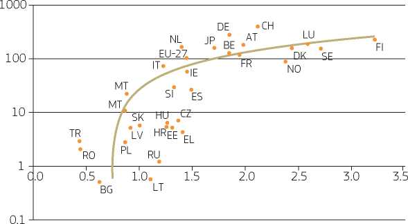
and R&D personnel as a share of total employment - 2005
Source: European Commission (2006)
The second step consists of providing an estimate of the patent portfolio that the RDI facilities will establish, as compared to a benchmark patent value.
For example, if the project’s RDI personnel is expected to register an average number of three patents per year and each of them is assumed to value EUR 100,000, the annual non-discounted benefit would be EUR 300,000. Given the high variability (and ex ante uncertainty) of the possible number and value of patents, different assumptions can be tested through the probabilistic risk analysis.
Knowledge spillovers to non-user businesses
RDI infrastructures can produce knowledge spillovers to non-user businesses. For example, if the RDI infrastructure is committed to developing new technologies (or goods, software, etc.) and releases them in the public domain without any form of intellectual property protection (e.g. because the RDI project promoter is a public entity), external users that use such technologies for their own sake would gain a benefit. The social benefit could be valued as the incremental shadow profit that the external business can be expected to accumulate thanks to the transferred technology.
Alternatively, instead of looking at increased profitability, in some cases it could be more practical to focus on avoided costs for businesses, which no longer need to develop the technology that has been made available for free (or at a very low price) by the RDI infrastructure.
The same approach would apply in the case of learning-by-doing benefits, which are enjoyed by high-tech suppliers involved in the design, construction or operation of infrastructures operating at the forefront of science (usually fundamental or applied large research facilities). Businesses which have the opportunity of acquiring new knowledge and technological skills spilling over as externalities from the RDI facilities may use such knowledge to produce further technological advancement and increase their sales performance and competitiveness. Even in these cases, the benefit could be captured by the change in shadow profit of non-user businesses attributable to the RDI project, or avoided costs.
This box presents an example of the valuation of knowledge spillovers to non-user businesses. All figures and assumptions hereby reported have a purely illustrative purpose and should therefore not be taken as reference values. The project proposer is invited to rely on project-specific assumptions and sources, and to duly justify the choice of any input value.
A public sector research project aims to find a new energy-saving process for the production of a given item and the project promoter is committed not to patent the research results. Only ex post it will be known if the project is successful; however, ex ante technologists may offer an estimate on the probability of the project being successful and a range of energy-saving results achievable (for example, due to preliminary evidence available through theoretical or pilot studies).
For instance, a RDI facility aims to investigate innovative combustion and gas turbine technology and offers open access to academic researchers and businesses. The results of experimentations are public and the project promoter envisages releasing information about the technological progress achieved through open conferences. Businesses that have not been involved in the experimentation process as users of the facility could still enjoy some benefit by absorbing the new knowledge produced by the RDI project that was released in the public domain. The new technology allows the businesses to significantly improve their own production processes.
The related social benefit will then be the avoided cost for each business to develop the same new/improved technology times the number of targeted businesses. In this case, if the application of the innovative technology allows the energy savings in the businesses’ production process to be achieved, then the benefit would be equal to the avoided energy cost for each business over a certain time horizon.
The value of scientific publications
For scientists and researchers, one of the main benefits of working within a research infrastructure, either for applied or fundamental research, is the opportunity to access new experimental data, to contribute to the creation of new knowledge and, ultimately, to publish scientific papers in scholarly journals. Thus, the unit benefit is the marginal social value of the scientific publication.
The marginal value of the publication can be estimated by its marginal production cost. This approach to account for benefits is entirely consistent with the standard approach described in Chapter 2, when marginal cost is a proxy of the shadow price of goods for which market prices are not appropriate.327
Thus the value of one paper in money terms may be estimated by the ratio of the salary of the author scientist over the number of publications per year. Other knowledge outputs, such as working papers, pre-prints and talks at conferences, can also be considered and valued according to the same marginal production cost approach.
The salary of the academic researcher should be considered only for the time dedicated to research. Data on the salaries of scientists and the average number of publications per year according to different scientific fields can be found in various data sources. Predicting the number of papers produced can be influenced by the standards of the personnel who are expected to be recruited for the research infrastructure.328
This box presents an example of the valuation of scientific publications. All figures and assumptions hereby reported have a purely illustrative purpose and should therefore not be taken as reference values. The project proposer is invited to rely on project-specific assumptions and sources, and to duly justify the choice of any input value.
In this example, the average gross salary of a scientist, who is a user of the RDI infrastructure, is EUR 60,000 per year, the time devoted to research is 50 % (the remainder being for teaching and managerial duties) and the number of published papers expected per year is three. The marginal cost per paper is then EUR 10,000: 60,000*50 %/3. For simplicity, a linear relationship between the value and the number of publications can be assumed and the total value of publications produced over the project’s time horizon can be estimated.
Additionally, whenever deemed relevant to the specific project, the value of the papers can be increased in proportion to the number of citations they receive by non-user academics who benefit from the new scientific literature created by the project users. Different approaches can be proposed by the project appraiser to forecast the dissemination process of scientific knowledge transfer through citations (e.g. by resorting to scientometric techniques) and to attribute a value to citations, provided that they are in line with the general principles of CBA. This additional effect could be important for fundamental and applied research infrastructures, while it is more limited and often negligible for innovation-focused infrastructures.
If scientists are expected to generate new patents, the same valuation methodology presented in the previous section applies.
The benefit of human capital development
The main benefit that could possibly be expected for junior researchers and students involved in the project is a ‘premium' to their future salary, resulting from the acquisition of human capital that would have not been accumulated without their participation in the project.
The premium is the incremental lifelong salary earned by young researchers and students over their entire work career, as compared to the without-the-project scenario. The estimation of such a future premium may require benefit transfer approaches from other contexts, interviews and expert opinion by specialists in the labour market of interest.
It is also important to note that a relatively small premium may accumulate over the years (for example during a researcher's 35-40-year career). For research infrastructures that attract many students or junior researchers, the aggregate value of the benefit may be non-negligible. This benefit would also be important for research and development laboratories of higher education institutions. Note that benefits produced beyond the project's time horizon should be included within the residual value of the analysis.
An equivalent and alternative approach would be to estimate the WTP for junior researchers and students to attend a training and study period at the RDI infrastructure. Similar to being admitted to prestige universities, students may be willing to pay a fee to access a research infrastructure, on account of the increased salary they expect to earn once they enter the labour market. The estimated WTP must be included in the economic analysis, in place of the financial revenues from student fees.
This box presents an example of the valuation of human capital development. All figures and assumptions hereby reported have a purely illustrative purpose and should therefore not be taken as reference values. The project proposer is invited to rely on project-specific assumptions and sources, and to duly justify the choice of any input value.
It is assumed that an applied research centre, operating for 20 years, hosts 100 students every year for a training period, for a total of 2,000 students. After their training period, former students are expected to immediately enter the labour market. Depending on the professional sector, the average gross annual salary can be easily derived from available national statistics or benchmarks from other similar contexts. In this example it is assumed that former students will earn an average annual gross salary of EUR 50,000.
Interviews with students, professors and other experts suggest that participation in the training programme offered by the research centre may generate a salary premium of, let’s say, 5 % over the total future salary as compared to the project-specific counterfactual situation (e.g. a training programme in another research facility or no on-the-job training at all). This corresponds to a non-discounted benefit of EUR 2,500 per year per student.
Assuming a work career of 40 years, the non-discounted benefit amounts to EUR 200 million: 100*20*2,500*40. The total discounted benefit can be estimated as the present value of the total annual incremental salary gained by all students trained during the project time horizon over their entire work career. Even after discounting, the benefit could still remain very significant.
To be more rigorous, one may decide to consider, instead of an average salary, the salary curve associated with students during their whole forthcoming work career. The graph below shows some examples for such salary curves. They refer to the expected salaries of doctoral students in the United States of America (USA), depending on the professional sectors of employment. Other sources may exist at European and national level. For example, the Annual Survey of Hours and Earnings329 of the United Kingdom’s Office for National Statistics provides the average pay for a large variety of professions.
Example of salary curve for USA workers in different professional sectors
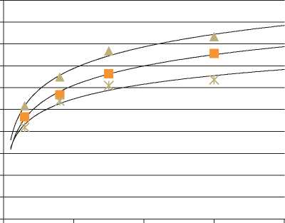
■ Industry
▲ Others (computing, financial, public administration, etc.)
X Academia and other research centres
0 10 20 30 40
Years of career
100,000 S 90,000
80,000
70.000
ru
S 60,000
50.000
40.000
30.000 < 20,000
10.000 0
Source: Authors’ elaboration based on PayScale data (www.payscale.com): the logarithmic function has been estimated from the expected salaries at four different career level.
The benefit of social capital development
There is an increasingly important academic literature in applied economics about the socioeconomic value of social capital, i.e. the dimension and depth of the network of relations among individuals. At this stage the literature is still in its infancy,330 but this potential benefit can be analysed by the project proposer in qualitative terms, without including its value in the calculation of the economic performance indicators.
Reduction of environmental risks
Some research infrastructures are focused on programmes that are intended to monitor certain classes of large-scale risk and to study mitigation measures. Different territorial risks may be in place. For simplicity, they are grouped here under the same label of environmental risk, where the ‘environment' concept is understood, in a broad sense, as the surroundings or conditions in which a person lives and operates.
Currently, the most encompassing risk for the human kind is climate change, and researchers are interested in understanding its dynamics and how to contain it. While this research may be conducted by relatively small scientific stations or expeditions, in some cases it may require coordinated networks of research facilities. Such networks can be considered as a unique major project if they are fully integrated, as discussed in section 7.4. Other classes of natural risks are, for example, soil erosion, floods, forest fires, earthquakes and volcanic activity. Technological risk for the environment is related to major pollution episodes in certain classes of economic activities.
When teams of people work at an applied research facility to test new methods of studying data related to potential environmental risks, to collect new evidence, elaborate forecasting models, possibly develop prototypes of new technologies and products aimed at reducing such risks, the ultimate beneficiaries of knowledge advances are potentially all the people at risk within the specific class of environmental risks considered.
The benefit of new knowledge in this area is the per capita avoided cost of the population potentially targeted or their willingness-to-pay for reduced environmental risk. There are some relatively well developed CBA methods for specific classes of risk that can be found in the literature of environmental economics (see section 4.3 on ‘Environmental remediation, protection and risk prevention'331 and Annex VI), most of them based on the calculation of the economic value, either of risk prevention or of the value of the damage arising from the occurrence of the accident and avoided thanks to the project. Double counting with possible financial revenues provided by the target population should be avoided.
The special difficulty for CBA in the context of RDI infrastructures is that, ex ante, it is unknown as to whether the project will be successful in providing new solutions over its time horizon. Two opposite scenarios could occur: a pessimistic scenario where nothing new or nothing of practical relevance is discovered, and an optimistic scenario in which the project entirely achieves its research objectives. Particular attention should be paid to avoiding unfounded optimism, deriving, for example, from imperfect information on unproven technology, a tendency of project developers to be over-optimistic and political incentives to be more optimistic to promote the project (see Table 7.8 at the end of this chapter for further examples of typical risks).
It is suggested that, as a baseline, the social benefits of the (carefully) optimistic scenario are calculated in the first place. In other terms, the project promoter should identify the measurable benefit to the target population of discovering what the infrastructure is reasonably intended to do. As mentioned, this can be done by relatively well-known techniques, at least for common environmental risks. Then the evaluator should consider the probability that the project is only partially successful and examine the risk affecting the ENPV through a fully-fledged risk assessment, including the risk of failure to discover anything applicable.
Reduction of health risks
One of the most important areas of contemporary research is related to human health, in such fields as, for example, the discovery and testing of new drugs, new advanced forms of surgery assisted by robotics, radiotherapy with non-conventional beams, genetics, etc. Research on the safety of the food chain or the safety of transport modes is also important to the perspective of human health.
In some cases such research can deliver results that are internalised by businesses (e.g. in the pharmaceutical industry, or in the production of electro medical equipment), by means of patents or other intellectual property protection systems. When benefits are fully internalised, then the businesses would be the main direct target group of the RDI project and the related benefit should be valued with the methods discussed in section 7.8.3 above.
In other cases, however, knowledge produced by applied research infrastructures is not appropriated by any specific business but it affects, directly or indirectly, the target population; for example, hospital research laboratories or other medical research facilities developing and administering a new type of treatment to their patients.
As with standard health projects, the project's marginal benefit is the reduction of mortality or morbidity rates or improved health conditions. They can be valued through the value of statistical life (VOSL), as discussed in Chapter 3 with reference to the economic cost of fatalities and accidents in the transport sector, of the quality adjusted life year (QALY) measuring the value of a change in both life expectancy and quality of life, or other statistical measures well known in health economics.332 In order to avoid double counting, any financial revenue coming from the targeted population should not be included in the economic analysis.
The evaluator will need to have the following:
• a forecast of the number of patients over the time horizon of the project;
• an empirical estimation of the marginal benefit (VOSL, QALY or others) for the target population that will be treated;
• a forecast of the success rate of the therapy.
The latter is obviously the most challenging aspect of the analysis, as, by definition, in medical research it is unknown whether a new treatment will work or not on a certain pathology and for a certain sample of patients. As with benefits to populations at environmental risk (see above), health benefits generated by the RDI infrastructure have to be forecasted and valued under a pessimistic and a (carefully) optimistic scenario. The probabilities of success, as well as the possible impact on the target population, can be inferred from relatively similar but more established medical treatments, and can rely on expert opinion collected through focus groups, interviews, Delphi methods and other techniques. This evidence, where it is necessary to get the patients' approval for experimentation, is likely to be available to the project promoter.
The economic benefit to the target population shall be estimated under the (carefully) optimistic scenario, but the risk that the research is not fully or partially successful should be assessed through the risk analysis.
Additional to the direct benefit of the population targeted by the RDI project, there could be another important benefit, which has to do with the public good nature of knowledge in medicine and related fields. While the treatment of each patient is not a public good per se (the individual therapy is to a certain extent rival and excludable), the knowledge acquired in a health research infrastructure can spill over to the world's medical community in various way: by publishing results, organising scientific congresses, hosting medical teams from other research centres, signing formal agreements for knowledge transfer (both for free or against a payment), etc. In these cases, there could be other indirect target groups, i.e. patients not treated at the research infrastructure, but who will be treated elsewhere due to the experience and discoveries cumulated by the initial project.
The marginal benefit and the evaluation approach is the same as for directly targeted populations. The scope of analysis, however, needs to be enlarged. This implies estimating the size of the wider target population, the possible impact on the wider population and the probability that knowledge transfer will occur. As usual, a probabilistic risk analysis will help to assess the overall variability of the resulting ENPV.
Cultural effects for visitors
Some RDI infrastructures attract the interest of the general public and their management may have an outreach strategy to this end. The reasons to design outreach activities for science and technology ventures could be related to increasing the social acceptance of large-scale projects that may otherwise be misunderstood by the general public and/or to ‘educate' people about what is carried out within the RDI facility. Examples of outreach activities could include the organisation of guided tours for visitors, for example, by the science park, or agreements between a research competence centre and schools and universities, aimed at arranging onsite educational programmes. There are many examples in Europe and in the USA of research infrastructures with large numbers of visitors per year, and project promoters may consider whether they want to develop such outreach programmes as part of their strategy.
The ultimate beneficiaries of these activities are the visitors to the infrastructure. Since visits are often free or at minimal prices, the marginal social value of the benefit is the visitors' implicit willingness-to-pay for a visit. As with other recreational activities, the most common way to estimate the WTP is through the travel cost method or benefit transfer approach (see the discussion in Annex VI). This means the evaluator would need to forecast the number of visitors in the time horizon of the project and to estimate the appropriate WTP. The WTP approach can also be used to value the sale of educational books or other publications aimed at disseminating knowledge to the general public. In the economic analysis, the WTP replaces the revenues from visitors included in the financial analysis.
Besides personal visits, there could be a number of virtual visitors, who will possibly visit the project's website or join social networks related to the project's activities. Some projects may also have some exposure in the media. When relevant, the project promoter shall attempt to evaluate the cultural benefits enjoyed by virtual visitors through appropriate CBA techniques, drawing from the increasing literature in cultural economics or, at least, in qualitative terms.
This box presents an example of the valuation of cultural effects for visitors to a RDI infrastructure. All figures and assumptions hereby reported have a purely illustrative purpose and should therefore not be taken as reference values. The project proposer is invited to rely on project-specific assumptions and sources, and to duly justify the choice of any input value.
In this example, the RDI infrastructure under appraisal is a competence centre specialising in developing technologies applicable to aircraft. The facility, besides being used by researchers, gives the general public the possibility to visit the laboratory on selected days of the month and to arrange demo flights for free. Approximately 100,000 visitors are expected to come every year during the project operation phase. No revenue from the visitors is recorded in the financial analysis, but their willingness-to-pay (WTP) should be accounted in the economic analysis to reflect the cultural benefit to the public. In line with the valuation of benefits associated with recreational goods (see section 4.3.7.3), the travel cost method333 is applied to estimate the WTP for a visit to the RDI centre.
Interviews with a sample of experts allows identification of where visitors possibly originate: in particular, 80 % of visitors are likely to come from an area within a radius distance below 150km, and 20 % from a longer distance. A further assumption needs to be made about the transport mode used by visitors. The WTP is reflected by the sum of the cost of a return ticket if travelling by train, bus or plane, or the cost of fuel, tolls and other operating costs if travelling by car, the value of time spent in traveling (e.g. using the HEATCO reference values for leisure trips, see section 3.8.1), the cost of meals and, for the share of visitors coming from a distance greater than 150 km, the possible cost of accommodation in a hotel. Only costs imputable to the visit at the RDI infrastructure should be included in the estimation of the WTP.
The average WTP for the different classes of visitors (coming from a shorter or longer distance and by different transport modes) is then multiplied to give the expected number of visitors per year in order to obtain a valuation of the economic benefit. For further details about the travel cost method, see Annex VI.
The above discussion about the valuation of benefits has not paid yet specific attention to the regional dimension of the possible impacts of the RDI infrastructures. This issue, which is obviously important in the context of cohesion policy, is discussed in this section.
In principle, all the benefits mentioned above can be given a spatial dimension, which is related to the location of identified target groups. The ubiquitous nature of research knowledge, however, implies that, in some cases, tracing the geographical boundaries of its impact has limited meaning. In other cases, however, it makes sense to ask the following question: to what extent is the region, where the RDI infrastructure is going to be located, expected to capture benefits from the project?
It is not suggested to break down in quantitative terms the project's net present value into local, regional, national or trans-boundary impacts. This is also not done for any other major projects discussed in this guide, and it would be an unnecessary analytical burden. However, the project proposer may consider offering some quali-quantitative evidence about the benefits and costs for the regions, at the appropriate scale (e.g. at NUTS 2, NUTS 1 or NUTS 0 levels). In some cases, the project could be expected to produce displacement effects in neighbouring regions, for example if it aims at attracting researchers previously employed in another existing RDI facility. It is suggested that the project proposer discusses significant displacement effects in at least qualitative terms.
The possible benefits and costs to be considered in a regional perspective are non-pecuniary and pecuniary externalities, the direct impact on regional competitiveness and other wider regional effects. The approach to evaluate them is discussed below. In general, the project proposer should be very careful to avoid double counting in the CBA.
Externalities
It is worth mentioning that there may be some social cost related to the infrastructure that is not captured by the financial analysis. These may be mainly environmental impacts during the construction, operation and decommissioning phases, such as air/soil/water pollution, GHG emissions and noise. Air pollution can be produced, for instance, by the increased number of vehicles coming to the RDI infrastructure. Another example is the release of some toxic substances, which can be expected from some infrastructures at the end of their lifetime.
Savings in energy consumption due to the building refurbishment and the implementation of energy efficiency measures could also be generated as a side effect of the project.334
While it is difficult to make general statements about the intensity and direction of environmental effects arising from RDI projects, if they are important to specific cases they must be valued and included in the CBA, following the methods discussed in other chapters of this guide (particularly Chapters 3 and 4 on the transport and environment sectors). In other cases, it is sufficient to mention and discuss them qualitatively in the project appraisal dossier.
The RDI infrastructure could also produce some (positive or negative) pecuniary externalities, particularly as regards the price of real estate and services, by affecting the demand for them. As suggested elsewhere in this guide, the change in property values can be assessed by hedonic prices (see methodological approaches in Annex VI and examples of application in Chapter 4). Since pecuniary externalities are to some extent captured by market price mechanisms, special care should be taken to avoid any double counting of benefits.
Direct impact on regional competitiveness
The direct impact on regional competitiveness is particularly appropriate for RDI infrastructures benefitting, in different ways, the enterprises operating in the region. From the CBA's perspective, as previously discussed, benefits are ultimately captured by increased profitability for the businesses, estimated in an appropriate way, including, when relevant, the expected value of patents. Clearly, from the regional perspective, the more these effects are captured by businesses located in the region the greater the impact on regional competitiveness.
Beyond a business's profitability, there may be other mechanisms that, albeit difficult to quantify, may be at least identified qualitatively. These include the attraction of scientists, technological experts and skilled personnel in general. The increase in the quality of a resident workforce has a long-term beneficial effect, by contributing to the cumulative process of building a favourable business environment. It is, however, difficult to give a monetary value without committing double counting with other benefits that are already quantified.
Personnel who were originally involved in the RDI project may, after some years, move to an occupation in one of the local businesses or start a spin-off company. In turn, this would reinforce the competitiveness of businesses and potentially attract other qualified personnel from elsewhere. From this perspective, it would be important for the project proposer to describe to what extent the project is expected to recruit personnel from other regions and other countries: a high rate of attraction to outsiders may be seen as an advantage for stimulating regional growth, but at the same time a social loss for other regions. As mentioned above, any significant displacement effect among regions should be duly accounted for in qualitative terms.
In a similar vein, the project may help to counteract the brain drain often suffered by some regions, by giving young local researchers or technical staff more employment opportunities. As usual, it is important to avoid double counting: the employment effects should be accounted for by the shadow wage of personnel recruited by the RDI project and no additional benefits need to be considered in the CBA. Thus, the number of jobs created or preserved for skilled personnel resident in the region should be provided as additional qualitative information.
A similar reasoning applies to the attraction of capital or of other businesses. Successful RDI infrastructures may be instrumental in conveying fresh capital from outside investors, which will find better investment opportunities in the region, more qualified personnel, and research and development facilities that are of interest to certain industrial sectors. This effect may also contribute towards increasing regional competitiveness. If some reliable forecasts about this possible effect exist, they should be provided, without having been accommodated in the CBA. For this reason, this particular effect should be discussed qualitatively and not considered for the computation of the ENPV.
Wider regional effects
The RDI infrastructure may have wider local effects on the regional context, which - as discussed in section 2.2 - shall not be included in the quantitative analysis, but better described in qualitative terms.
First, there may be demonstration effects on the general population, particularly the young, about the role of science and technology. While some of these effects may be captured by the cultural effects on the general public, included in the CBA, as mentioned above, others may be more subtle. For example, the proximity of schools and universities to a RDI project may convince a larger share of students to study engineering or to achieve a degree in sciences and this, in turn, could be somewhat correlated to the long-term regional growth rate.
Second, as science parks, laboratories, competence centres in the high-tech sector, etc. attract high quality personnel, possibly from other regions or abroad, these may contribute to opening the cultural horizon of the local society. This in turn contributes to an increase in local social capital and in some particularly beneficial cases, even to the improvement of the overall quality of institutions. Academic research in this area is still not sufficiently mature for practical applications. However, if the project promoter guesses that there will be such future effects, caused by an inflow of international, highly qualified migrants, this may be stated in qualitative terms. Some supporting evidence about the likely numbers and origins of the new residents shall be provided.
While the focus of this chapter is on applied research, development and innovation infrastructures, it is briefly mentioned here that the previously examined benefits may not be the core ones from the perspective of fundamental research infrastructures. Discovery per se (e.g. the discovery of a new elementary particle, a new biotype or natural species, a new exoplanet, etc.) is often the primary objective of a fundamental research infrastructure. However, the social value of pure discovery is an entirely new field for CBA and its possible valuation methodology still represents a challenge.
One possible evaluation approach could resort to concepts gathered from the CBA of environmental projects, which may also be relevant to fundamental research projects. For example, the notion of quasi-option value, i.e. the social value of future potential applications stemming from fundamental research which at present are not yet well identified,335 could be relevant in the fundamental research context.
There is much more experience in estimating the existence value of environmental and cultural goods (Annex VI). This refers to the benefit for an individual from just knowing that a certain good is preserved for future generations or, in the case of research, that something new is discovered. Empirically, the existence value of goods can be estimated by contingent valuation. In 1993, the USA's National Oceanographic and Atmospheric Administration released a very influential guideline on contingent valuation of the existence value, based on the recommendations of a panel of high-profile experts. In the EU, there is no extended CBA experience in this area yet, but research on the topic is ongoing.336
The probability of error related to each estimate included in the above analysis could be particularly high from an ex ante perspective. While this is true in general terms for any infrastructural project, in the case of RDI infrastructures the overall uncertainty of CBA results can be even larger.
In order to deal with the intrinsic project riskiness and uncertainty about some input variables, a fully-fledged quantitative risk assessment is required. With reference to section 2.10, this should comprise a sensitivity analysis (completed with a scenario analysis), a qualitative risk analysis, a probabilistic risk analysis, and the definition of a risk prevention and mitigation strategy.
The following list shows the variables that are likely to be critical and which should be tested in the sensitivity analysis, as well as duly considered in the qualitative analysis through the risk matrix:
• number of years necessary for the construction of the infrastructure;
• investment and operating cost items;
• licence revenues gained from patents' commercialisation;
• revenues from the target population using the research outputs (e.g. patients receiving an innovative treatment);
• revenues from outreach activities to the wider public (e.g. bookshop sales, entry fees, etc.)
• national/regional funding schemes for RDI activities;
• public grants to research;
• number of spin-offs and start-ups expected to be established;
• spin-off equity realisations;
• expected annual incremental profit earned by spin-offs and start-ups;
• survival rate of spin-offs/start-ups;
• expected incremental shadow profit;
• number of patents expected to be registered over the project time horizon;
• economic value of patents;
• number of non-user businesses benefitting from technological spillovers;
• expected incremental profit earned by businesses that benefit from technological spillovers or avoided costs;
• number of scientific publications expected to be produced over the project time horizon;
• estimate of the unit economic value of scientific publications;
• average number of citations received by scientific publications;
• number of young researchers and students benefiting from human capital development;
• expected incremental salary obtained by students as a result of human capital development over their professional career;
• size of targeted population at environmental risk;
• avoided cost or WTP for reduced environmental risk;
• forecast of the success rate of the project;
• size of targeted population at health risk;
• VOSL or QALY;
• forecast of the success rate of the project;
• estimated WTP of visitors;
• estimated WTP for educational publications;
• value of environmental impacts;
• hedonic prices.
The sensitivity analyses allow for the identification of the most critical variables of the CBA model. The probability of change for the CBA results (in terms of net present value and internal rate of return) against simultaneous changes of the critical variables, according to their own probability distribution functions, should be tested.337 Unlike the major projects that fall under other sectors, where the implementation of the probabilistic risk analysis is only recommended in some cases, this type of analysis should be regularly included in the appraisal report of RDI infrastructures. Monte Carlo simulation techniques should be employed in order to judge the project risk in probabilistic terms.
As described in section 2.10.4, the final step of risk assessment procedures consists of defining a risk prevention and mitigation strategy for the proposed project. The typical risks affecting RDI infrastructure projects, and which should be explicitly taken into account, are listed in the table below.
Table 7.8 Typical risks in RDI projects
|
Stage |
Risk |
|
Demand analysis |
- Evolutions in the labour market (demand for university graduates and an impact on the demand for education services in the area) - Insufficient qualified human resources for research activity - Demand of students different than predicted - Demand of industrial users different than predicted - Interest of the general public different than predicted |
|
Design |
- Inadequate site selection - Inadequate design cost estimates - Delays in completing the project design - Invention of a new RDI technology making the infrastructure’s technology obsolete - Lack of well-established technical engineering expertise |
|
Administrative and procurement |
- Delays in obtaining building permits - Unresolved property ownership rights - Delays in the acquisition of intellectual property rights or higher-than-expected costs for their acquisition - Procedural delays to select the supplier and sign the procurement contract - Supply bottlenecks |
|
Construction |
- Lack of ready-made solutions to meet the needs arisen during the construction or operation of the infrastructure - Project cost overruns - Delays in complementary works outside the project promoter’s control - Project delays and cost overruns during installation of scientific equipment - Accidents |
|
Operation |
- Unexpected complication connected with the installation of specialised equipment - Delays in making the equipment fully and reliably running - Insufficient production of research results - Unexpected environmental impacts/accidents - Lack of academic staff/researchers |
|
Financial |
- Inadequate estimate of financial revenues - Insufficient success in obtaining national and international competitive funding - Failure to meet the demand of users - Inadequate system for protection and exploitation of intellectual property - Loss of existing clients/users due to competition from other RDI centres |
Source: Authors
This box presents an example of probabilistic risk analysis. All figures and assumptions hereby reported have a purely illustrative purpose and should therefore not be taken as reference values. The project proposer is invited to rely on project-specific assumptions and sources, and to duly justify the choice of any input value.
This example assumes that a RDI infrastructure project, consisting of the construction of a technology park for applied research and innovation, has an economic net present value of EUR 400 million over a 15-year horizon (baseline scenario). The main economic benefits come from the generation of start-ups and the value of new products developed by user companies, which are ready for commercialisation. High uncertainty, however, affects the assumptions at the basis of the benefit valuation, which mainly rely on interviews with future user businesses and benchmarking with similar facilities in the same country.
A sensitivity analysis is carried out to identify the critical variables of the model, with particular reference to the economic analysis. A 1 % change in the value of the majority of the CBA inputs (related to investment costs, revenues, operating costs and economic benefits) is considered. Those variables that lead to a greater than 1 % change in the ENPV are:
- on the cost side, the construction cost;
- on the benefit side, the number of new start-ups generated;
- the shadow profit expected to be produced by existing businesses from the commercialisation of the innovation products.
Construction costs
mean = EUR 80 million
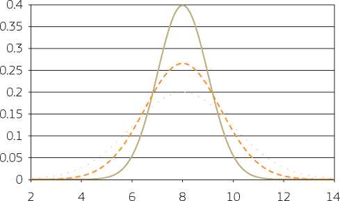
sd = 1 ---sd = 1.5 sd = 2
Number of start-ups min = 5, mode = 20, max = 25
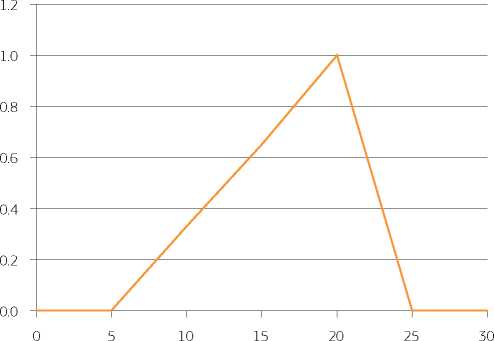
In parallel to a qualitative risk analysis, carried out by means of a project risk matrix (not discussed here but see Chapter 2), a probabilistic risk analysis is implemented.
As a first step, a probability distribution is assigned to each of the critical variables identified through the sensitivity analysis. Three different distributions are assumed for each variable.
In the baseline scenario construction, costs have been estimated at EUR 80 million, split over five years. Acknowledging that a number of factors may intervene to change the total construction costs, after consulting with experts the project promoter assumes that the construction cost could change according to a normal distribution with a standard deviation equal to 1 (but different assumptions could have been made in this regard, see figure below).
As to the number of start-ups generated by the incubator available in the technology park, the baseline scenario considers that a total number of 20 businesses are established over ten years, but this variable is critical for the model. Benchmarking with other technology parks in other regions suggests that, while it would be possible for the project to support up to 25 new businesses, given a number of factors (e.g. uncertain availability of venture capital, limited number of entrepreneurs, etc.) it is more probable that a lower number of start-ups will be established, but anyway not lower than five. Hence, the project promoter has been quite optimistic in the baseline scenario. To simplify the computation, the discrete distribution of the number of start-ups has been taken as continuous, and reflected in a left-skewed triangular distribution.
The RDI project allows already-existing businesses to benefit from the use of testing and prototyping laboratories, which eventually lead to the development of new marketable products. Due to some unemployment in the region, the conversion factor for labour is estimated at 0.8; thus the shadow profit gained by businesses for selling the innovation products differs from the financial profit.
Annual shadow profits
min = EUR 5 million, max = EUR 20 million
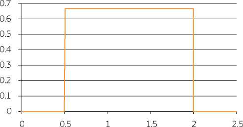
ENPV
(thousand EUR)
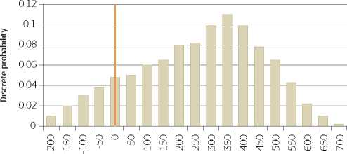
Expected annual shadow profit is highly variable. In principle, other variables are likely to be critical, such as the number of user businesses, or the time at which new products are actually developed, or the number of innovative products developed. Here for the sake of simplicity and example, only the annual shadow profits are tested. Given the high uncertainty about this variable, the project promoter assumes that profits may take any value between EUR 5 million and EUR 20 million per year, while in the baseline scenario a EUR 15 million annual shadow profit has been assumed for any new product brought to the market. Thus, a rectangular distribution can be hypothesised.
Information about the probability distribution of critical variables is entered in computation software for a Monte Carlo simulation. Through the software, a set of values for the three above-mentioned critical variables are randomly extracted within their respective defined intervals and probability distribution functions.
A total of, let’s say, 1,000 extractions are made. The economic net present value resulting from each set of extracted values is estimated, so as to obtain a probability distribution of the performance indicator, shown in the graph below.
Due to a certain optimism bias in the assumptions behind the number of start-ups and the annual shadow profit enjoyed by existing user companies, once considering the probability distribution functions of critical variables, the mean ENPV can be expected to be lower than the value obtained in the baseline scenario (EUR 400 million). Actually, in this example there is an almost 70 % probability that the ENPV will be lower than what was initially estimated and a 10 % probability that it will be negative. The risk analysis suggests that proper mitigation measures, focused on specific variables, should be taken to ease the materialisation of benefits.
When investors, either private or public, commit capital to a project, they have an implicit cost deriving from sacrificing a return to another project. In other terms, the resources employed have an opportunity cost. Thus, to induce the investment, the expected return should be at least as high as the opportunity cost of funding. This is why inflows and outflows of a project are discounted by means of a financial discount rate (FDR).
The FDR is the opportunity cost of capital and is valued as the loss of income from an alternative investment with a similar risk profile. It takes into account the time value of money, for example the idea that money available now is worth more than the same amount of money in the future because it could be earning interest (in a non-risk deposit), and the risk of the anticipated future cash flow being less than expected.
Different approaches exist in the practice of calculating the financial discount rate.
• A commonly used approach consists of estimating the actual cost of capital. A proxy for this estimation is represented by the real return on government bonds (the marginal direct cost of public funds) or the long-term real interest rate on commercial loans (if the project needs private finance), or a weighted average of the two rates (Weighted Average Capital Cost - WACC). The latter case is applied, particularly, when a project needs the financing both of public and private funds. Although being very practical and widespread, this approach does not reflect the actual opportunity cost of capital, because the best alternative investment should, in principle, produce higher earnings than the interest rate paid on public or private loans.
• A second, more accurate, approach is to consider the return lost from the best alternative investment in order to determine the maximum limit value for the discount rate. In this case, the alternative investment is not the buying back of public or private debt but is the return on an appropriate portfolio of financial assets.
• Finally, the FDR is determined by using a specific interest rate or a rate of return from a well-established issuer of securities in a widely traded currency and then applying a multiplier to this minimum benchmark. Given the volatility of the international financial markets (including the risk of asset bubbles), however, this approach can lead to unstable and frequently changing values.
In the following, an empirical example for the calculation of the FDR in a small open economy is proposed by following the second approach. The calculation, made for illustrative purposes, deviates from the 4 % proposed in the main text as reference for the 2014-2020 programming period (which remains, as mentioned, an indicative benchmark value to be used for EU Member States in general).
The main underlying assumption is that the project proposer is an experienced investor and is able to obtain a return from his/her investment that is at least equal to the average value of a portfolio of different securities. The starting point for the estimation of the opportunity cost should be, therefore, the rate of return on the most common assets from which an investor can earn interest, namely government bonds, cash equivalents and stocks. This approach assumes that domestic and international security markets are integrated, meaning that there are no barriers to financial flows and that assets with the same levels of risk command the same return no matter the country. This is particularly suitable for small open economies, where the domestic returns on capital are less relevant than a diversified portfolio available on the international capital market338' As a consequence, even if the project is related to its country context, the estimation of the opportunity cost of capital can rely on an international portfolio of assets on the basis that the investor might commit his/her resources elsewhere'
In this example, one rating agency's estimates of long-term returns of an international portfolio of investments have been considered (see table below). The FDR is calculated as the mean339 of the returns from the assets included in the portfolio. The Fisher Formula340 is then used to get the real return estimates. Adopting these estimates, the calculated FDR is 2.9 % in real terms or 5.1 % in nominal terms.
Table I.1 Nominal and real return estimates
|
Asset class |
Nominal annual return estimates % |
Real annual return estimates % |
|
Large-cap stocks |
6.5 |
4.3 |
|
Mid-/small-cap stocks |
8.0 |
5.8 |
|
International stocks |
6.3 |
4.1 |
|
Bonds |
2.6 |
0.4 |
|
Cash investments |
2.2 |
0.0 |
|
Simple average |
5.1 | |
|
Long-term inflation rate |
2.2 | |
|
Simple average |
2.9 |
Source: www.schwab.com
The social discount rate (SDR) is used in the economic analysis of investment projects to discount economic costs and benefits, and reflects the opportunity cost of capital from an inter-temporal perspective for society as a whole. In other words, it reflects the social view of how future benefits and costs are to be valued against present ones. In this sense, every discount rate entails a judgement concerning the future and it affects the weight attributed to future benefits or costs.
A zero social rate of time preference derives from the assumption that equal weights are given to the utilities occurring at any moment, i.e. that today's and future consumptions are indifferent to the utility point of view. A positive discount rate, on the other hand, indicates a preference for current over future consumption, whereas the opposite is true if the discount rate is negative.
In a perfectly competitive economy and under equilibrium, the social discount rate coincides with the financial discount rate, which would correspond to the financial market interest rate. However, this does not apply in the practice, since capital markets are in fact distorted.
Different approaches have been proposed by the literature to estimate the SDR. The most popular ones are provided here.
• The social rate of return on private investments (SRRI) is based on the idea that public investments displace private investments. Therefore, according to this approach, the return from the public investment should be at least as big as the one that could be obtained from a private investment. As a result, the SDR is considered equal to the marginal social opportunity cost of funds in the private sector. As mentioned by many economists (Boardman et al., 2006, Barrett et al., 1999, Arrow and Lind, 1997), the SRRI approach is generally biased toward high estimates of the SDR. There are two main causes of this bias: first, externalities and market failures distort private investment returns and may generate private investment returns higher than the social ones; secondly, the observed private return on investments usually includes a risk premium. This is however not to be included in the SDR because society as a whole, or the government, has a much larger portfolio than any private investor has and consequently is able to exploit risk pooling. As an empirical estimation of the SRRI is typically based on observed returns in the private financial markets, one additional concern here is market volatility and the role of asset bubbles.
• The social rate of time preference (SRTP) is the rate at which society is willing to postpone a unit of current consumption in exchange for more future consumption. The logic of this approach is that the government should consider the welfare of both the current and future generations and solve an optimal planning programme based on individual preferences for consumption. Different methods exist to estimate the SRTP. First, it can be estimated by looking at the return on holding government bonds or other low risk marketable securities. Another way is based on a formula obtained from the Ramsey growth model (see below). A possible limit of the SRTP approach is that, by focusing on the consumption side, it disregards the displacement effect that public projects might have on private investment. Lind (1990), however, maintains that, because of international capital mobility, the crowding out effect of private investment by public investment does not appear to be very important to the analysis of the social discount rate.
• Other approaches exist and could be used for inter-temporal discounting, although they are rarely applied in practice. Among these are the weighted average approach and the shadow price of capital approach. The former implies that, when public investment is considered to have a displacement impact on both private investment and future consumption, the SDR could be estimated by a weighted average of the investment rate of return and the rate of time preferences. The latter entails the conversion of investment flows into ‘consumption equivalents' through an appropriate shadow price of capital; these flows are then discounted at the social rate of time preference.
The following table synthetically presents the SDR approaches currently used in selected countries worldwide. It can be
noted that the social rate of time preference method is widely used in developed countries, especially European ones.
Indeed, according to most economists (e.g. Feldstein, 1972, Evans and Sezer, 2003, 2004 and 2005, Florio, 2007, Evans, 2007, Kula, 2002 and 2006), this approach is grounded on a robust theoretical basis, as it does not rely merely on financial data but, above all, on social preferences.
Table II.1 Social discount rate methods as adopted in selected countries
|
Theoretical basis |
Country |
Source |
|
SRTP |
Denmark |
Hepburn (2007) |
|
France |
Quinet (2007) | |
|
Germany |
Florio (2006) | |
|
Italy |
Florio (2006) | |
|
Portugal |
Florio (2006) | |
|
Slovakia |
Hepburn (2007) | |
|
Spain |
Florio (2006) | |
|
Sweden |
Hagen et al. (2012) | |
|
United Kingdom |
HM Treasury (2003) | |
|
USA (Environmental protection Agency) |
Zhuang et al. (2007) | |
|
SRRI |
Australia |
Harrison (2010) |
|
Canada |
Guidelines of the Treasury Board secretary (2007) | |
|
India |
Zhuang et al. (2007) | |
|
Ireland |
Florio (2006) | |
|
Netherlands |
Florio (2006) | |
|
New Zealand |
Zhuang et al. (2007) | |
|
USA (Office Management and Budget) |
Zhuang et al. (2007) | |
|
Weighted average approach |
People’s Republic of China |
Zhuang et al. (2007) |
|
Government’s borrowing rate |
Czech Republic |
Hepburn (2007) |
|
Hungary |
Hepburn (2007) |
Source: Authors
The social rate of time preference
A relatively easy and largely used way to estimate the SRTP is based on the following formula, which is obtained from the Ramsey economic growth model (1928):
SRTP = p + e * g
where p is the pure time preference, e is the elasticity of the marginal utility of consumption, i.e. the percentage change in individuals' marginal utility corresponding to each percentage change in consumption; g is the expected growth rate of per capita consumption.341 The two components of this formula (the one related to time preference and the other related to consumption growth) reflect the two possible reasons why future consumption may have a lower value than in the present. First, present income or consumption is usually preferred because of uncertainty about the future and impatience. Second, future consumption may be valued at less than the present one because of the probability of people becoming richer in the future. Indeed, if per capita consumption is growing, then the value of additional consumption for each year in the future is declining at a rate related to the rate of growth of per capita consumption and the elasticity of diminishing marginal utility of consumption.
Each term in the formula is discussed in more detail below.
The pure time preference term (p) can be decomposed into two elements, one related to individuals' impatience and myopia, and the other one related to the risk of death or human race extinction. This latter component reflects the life chance and it is often simply measured as the ratio of total deaths to total population. The former component instead refers to the observation that individuals favour the present over future consumption and this is reflected in a positive value of p. However, as put forward by Ramsey and others, from a social perspective it is ‘ethical indefensible' to set this term different from zero (Ramsey, 1928, page 543). A positive value, actually, would signify that future generations are made worse off but only due to the fact that they are born later, which would be unacceptable from the point of view of society as a whole.
The economic empirical literature generally estimates a value for p of between 1 % (e.g. Newbery, 1992, Arrow, 1995, Evans, 2007) and 3 % (Nordhaus, 1993). However, in the Stern Review a 0.1 % rate is considered due to the assumption about a nil impatience or myopia component, in line with the above-mentioned Ramsey's argument.342 As a result, an easy way to proxy p could be to set the impatience or myopia component equal to zero and the risk of death or human race extinction equal to the annual crude death rate of the population (number of deaths over population).
The elasticity of the marginal utility with respect to consumption (e) captures the dynamics of consumption over time. This parameter captures the fact that if tomorrow consumers are a bit richer, marginal utility is decreasing. In other terms, it reflects how consumption should be transferred across different generations; it can be seen as a planning parameter for the social planner in that it reveals his preference for income inequality aversion.
An approach to estimate the elasticity term is to consider the social judgement about how consumption should be transferred across people at different times. In this case, the elasticity tells us how much more worthwhile it is to transfer income from a rich person to a poor one. This can be revealed by analysing the progressivity of national personal income tax rates. Stern (1977), Cowell and Gardiner (1999) and Evans (2006) propose the following formula of elasticity:
e = ln(l — t') /ln(l — t)
where t and t are respectively the marginal and average income tax rates for an average taxpayer.
One is the neutral value of the parameter: when e = 1, then EUR 1 of additional future consumption adds EUR 1 to social welfare. If instead e < 1, consumers are not so interested in future growth. If e > 1 consumers are interested in it.
The expected per-capita consumption growth (g) or other welfare-related variable (e.g. income, as stressed by Spackman, 2007 and Kula, 2012). From the point of view of inter-generational equity, this term implies that if future generations are expected to be wealthier that the ones of today, and thus if consumption rises over time, this would result in an increase of the discount rate in order to shift the priority to the poorer current generation. Usually very long-run growth rates of real per capita consumption are used to estimate future growth, in order to smooth out possible short-term distortions.
Empirical estimates for the rate of growth of per capita consumption are usually based on growth models, which take into account both the past long-term development path and the expected future growth. A way to estimate g is to consider another welfare correlated indicator as proxy for consumption growth, such as real per capita GDP growth, consumption growth or personal income growth.
As far as empirical estimation is concerned, the most recent evidence estimating the SDR for 20 European countries is presented in Florio, 2014 (see Bibliography).
For the purpose of the financial analysis, market prices represent a relevant signal for both the private and public investor when assessing the project's financial performance. However, they are no longer relevant when the aim is to assess the project contribution to economic welfare. For this purpose, all revenues and costs considered when appraising the financial performance (in particular those included in the tables for the assessment of the financial return on investment) and valued at prices observed on the market, have to be valued at the so-called ‘shadow prices'. A shadow price is the social marginal value of an output or input change, i.e. the opportunity cost to the society of producing or consuming more or less of any good.
Market prices and shadow prices are the same in perfectly competitive and efficient markets or under optimal planning. In reality, however, the markets may be distorted by taxes, duties, subsidies, rigid exchange rates, rations on production or consumption, regulated tariffs, oligopoly or monopoly price setting and imperfect information. These are elements that drive a wedge between the observed price and the marginal social value of resources.
- A land-intensive project, e.g. an industrial site, where land is made available free of charge by a public body, while it may otherwise earn a rent.
- An agricultural project that depends upon a water supply at a very low tariff, which is heavily subsidised by the public sector and where output prices are affected by special policy regimes (e.g. under some provisions of the EU’s Common Agricultural Policy).
- An energy intensive project that depends upon the supply of electricity under a regime of regulated tariffs, when these tariffs are below long run marginal costs.
- A power plant under a collusive oligopoly regime, which determines a substantial price divergence of electricity prices from long term marginal costs, the former being higher than the latter; in this case economic benefits could be less than financial profits.
The general theoretical framework of cost-benefit analysis is provided by Dreze and Stern (1987, 1990343), who estimate shadow prices as the net impact on the social welfare function of a unit increase of an input or output.344
There is no unique way to calculate the shadow price, which fits all types of market and non-market goods. Instead, several approaches exist, and each of them could be more or less suitable for certain typologies of goods and sectors (see Figure 2.2 in Chapter 2).
In order to apply the most appropriate method, a first important discrimination is whether the good is an input or an output of the project. For the latter, the willingness-to-pay approach described in Annex VI can be followed. As far as inputs are concerned, they can be regarded as tradable or not in international markets. The general rule for internationally tradable goods, such as most manufactured commodities, is to use their border price. As far as non-tradable goods are concerned, a different approach is followed, depending on the event of considering minor items or major items. For minor items, a special parameter called standard conversion factor (SCF) can be used.
Shadow prices for major non-tradable inputs depend on the effect that a demand or supply change for that good has on social welfare; these effects, in turn, depend on how the markets adjust to those demand or supply changes. In particular, the opportunity cost of project inputs whose use would lead to an increase in production must be estimated through the long term marginal cost345 of producing one additional unit of that input. Instead, when the use of an input will not result in increased production but in a reduction of consumption by alternative users, the willingness-to-pay must be estimated by reference to their social value, rather than to their cost. The shadow price in these cases is the price that alternative users would be willing to pay to consume that good.346
Labour cost represents an exception. Even if labour is characterised by freedom of movement across the EU, it cannot be considered a tradable good in the strictest sense. It is also valued differently to other non-tradable inputs: a specific shadow price (i.e. the shadow wage), which accounts for local distortions in the labour market, must be computed to determine its opportunity cost.
The different approaches for the empirical estimation of conversion factors to move from observed to shadow prices are presented in more detail below.
The border price rule is generally used to estimate shadow prices of internationally marketable goods entering as inputs in the project. It is gathered from the Little and Mirrlees (1974)347 approach to project evaluation. This approach, derived from research commissioned by the OECD, the United National International Development Organisation (UNIDO) and the World Bank, has been conceived for evaluating investment projects in distorted markets, such as those in developing countries. However, the same rules are relevant to any open economy, regardless of the degree of price distortion.
The border price method is based on the estimation of the trade opportunity cost of goods, under the assumption that international prices reflect the economic value of imported goods better than domestic prices. According to the border price rule, the shadow price of a tradable good is given by its CIF (cost, insurance and freight) price at the national border, thus including the cost of production, insurance and freight borne to bring the good as far as the national border, but excluding any custom duties, taxes or subsidies applied once the good enters the national market. These can be a percentage of the price of the good, a fixed amount per unit or a minimum price applied as the good passes the border.
The Little-Mirrlees rule applies to goods that are tradable by nature, for which an international market exists: these are typically most raw and semi-raw materials, manufactured goods but also some public utilities (e.g. natural gas supply). Conversely, transport services, civil works, maintenance costs, land, local transport and some other public utilities (e.g. water supply) can be considered non-tradable goods and for them the border price rule cannot be used.
In general terms, it can be stated that the border price rule can be applied whenever the next best alternative of domestic production is importing it. Hence, whenever international trade represents a feasible opportunity, border prices can be taken as shadow prices in the economic analysis of investment projects. This means that the rule can also be applied to goods that, in spite of being potentially tradable on the international market, are currently not traded in practice, for example because of low domestic attitude towards foreign trade.
For example, assume that a given good is produced in country A at a certain cost and in country B at a lower cost. A could decide to continue producing the good in spite of having the possibility of importing the good from B at a relatively lower price. Its shadow price will be the price of the next best alternative of self-producing the good. Since trading in principle is possible (e.g. a road linking country A and B exists) and would be financially more convenient (the import price would be lower than the production costs in A), importing the same good from B would represent the next best alternative for country A. Hence the shadow price of this good would be its border price.
Another main assumption for using the border price as the shadow price of a commodity in a country is that the world price of that commodity is fixed, i.e. it is not affected by significant variations in demand and supply in the national market. This assumption can be considered to hold in relatively small countries, whose domestic market changes cannot directly affect international markets, and when no particularly large investment projects are under implementation. In fact, ‘economically significant' or ‘mega' projects are such that they could influence national trade flows and, thus, relative prices. When these conditions are not met, shadow prices of imported items could be better proxied by following alternative approaches (see below).
The economic value of non-tradable inputs, for which an increase in demand results in increased production, can be measured by the marginal social cost of production. This method can be applied when the cost structure is known or can be easily identified, otherwise the standard conversion factor could be applied as a shortcut.
The marginal social cost of a good is the market price of the inputs required to increase the production of a good by one unit, less the social value of the extra profit for selling the extra good, holding the production levels of all other goods constant.
Variations in the long run marginal cost (LRMC) can capture changes in both operating and capital costs. By reflecting the marginal costs involved in providing an additional good, which enters as an input of the project under assessment, the LRMCs can be taken as a good proxy of the economic value of that good and, thus, can be used as the shadow price.
In calculating the LRMC, the project appraiser should consider, in principle, not only the incremental financial operational and capital costs involved when increasing marginal production, but also other environmental and non-market costs contributing at forming the total economic value of the good.
Estimating the LRMC can be arduous, as it requires detailed information on the structure of production costs, which could not be available to the project appraiser. Two general rules for marginal cost estimation can be provided. First, the LRMC should include on the operating and capital side only the actual extra cost of creating increased capacity required to meet the needs of the project. It is possible that not all costs necessary for production will need to be incurred to allow increased supply; for instance, some existing capital facilities may be able to cope with new productive capacity. Second, it should be considered that marginal cost pricing is a forward-looking concept, meaning that it should be based on the expected development in the cost structure. Furthermore, it could be useful to have in mind that LRMCs are generally lower than average total costs due to fixed costs and economies of scale, which characterise many businesses.
The LRMC of water should take into account the increase in costs led by an increase in water consumption (because of the project’s construction and operation activities), as well as the costs associated with the provision of new water resources, treatment capacity and any other costs that may occur in the long run. These include costs sustained to avoid or mitigate potential negative externalities, such as pollution, and the opportunity cost of the resource, in compliance with Article 9 of Directive 2000/60/EC.
More specifically, in the case of the economic cost of water, the LRMC can be computed as the sum of the cost categories listed below.
- Supply costs: they are based on the unit cost of the resource required by the investment project, calculated as the annualised capital and operating costs associated with the provision of water (from groundwater, surface water, desalinisation, etc.) divided by the volume of water consumed. Capital costs should also include any investment costs aimed at improving the water quality and the water supply system performance (e.g. by reducing losses and pollution, improving reliability, etc.).
- Treatment costs: they can be estimated through the annualised unit cost of the relevant sanitation and treatment process.
- Distribution costs: they include the annual unit costs (total distribution costs over the total volume of water distributed) of installing and maintaining the connection from the customer’s property to the mains and the specific costs related, e.g. to the pumping head, dams, the lengths of mains required, the soil types, desalination (depending on how water is gathered). These costs are generally differentiated by type of users, namely industry, households and agriculture.
- Other annual costs of service management, which include the cost of meter-reading, billing, keeping customer records and dealing with enquiries and other administrative costs.
- Any environmental costs associated with water supply and treatment, such as the social cost of pollution generated by the electricity used for pumping water, noise and environmental damages provoked during the construction phase, etc.
- Finally, the resource costs, i.e. the opportunity cost of using water for the project, to be valued in terms of the best alternative use of the resource.
Directive 2000/60/EC recommends water-pricing policies to take account of the principle of recovery of all the costs of water services, including financial, environmental and resources costs. Hence, whenever there is a guarantee that the water tariff is set in such a way as to ensure the full recovery of costs, particularly in accordance with the ‘polluter pays’ principle, the water tariff would equal its LRMC and can thus be taken as the proper shadow price of water.
Minor non-tradable items are inputs that do not represent a significant share of the project total costs and for which no sufficient information on their cost structure is generally available, thus impeding an estimate of their long term marginal cost. An adjustment method to estimate shadow prices of these items consists of computing the so-called standard conversion factor (SCF). The SCF is a proxy of the average distance between world prices and domestic prices, under the assumption that the former reflects the opportunity cost of the good and that the latter is distorted compared to international prices (in line with the border price rule). The lower the distortion of the domestic market, the closer the SCF is to unity.
Even if the gap between domestic and international prices can be determined by a wide variety of distortions, the most widely used formula to estimate the SCF takes into account only taxes and subsidies on trade as factors driving a wedge between market and shadow (i.e. international) prices. This is clearly a simplification, but it guarantees an easy applicability of the method.
The full formula generally used to estimate the SCF is:
SCF =
M + X
(M + TM — SM) + (X — Tx + Sx) where:
M is the total value of import at shadow prices, i.e. CIF prices;
X is the total value of export at shadow prices, i.e. free on board (FOB) prices;
Tm and TX are the value of duties on import and export respectively;
SM and SX are the value of subsidies on import and export respectively.
Like the border price rule applying for estimating the shadow prices of tradable goods, the CIF prices at the national border are taken as a proxy of the international value of imported good. The FOB prices are taken as a proxy of the international value of exported goods, including the cost of production of the goods and their transport up to the border, before any subsidies or taxes are applied for them being exported.
In a multi-level government such as the European Union, observed prices should also be free of custom duties (and any subsidy) levied by the EU imports entering each Member State from third countries. Additionally, in Member States that have both central and sub-central levels of governments, taxes and subsidies imposed by each of these levels should be taken into account.
The general formula for the SCF can be simplified if no taxes or subsides are levied either on imports or exports. In computing the SCF for the EU Member States, in particular, some considerations can be made:
• some taxes and duties are generally levied by the national governments (at both central and sub-central level) on imports from other countries and by the institutions of the European Union for imports from non-EU countries;
• import subsidies are usually not a practiced measure by either EU institutions or national governments;
• exports to other Member States and third countries are generally free of taxes;
• subsidies linked to the volume and value of exports are, in principle, not granted by both the EU institutions and national governments, in line with the 1994 World Trade Organization (WTO) agreement. However, in spite of an actual fall of export subsidies in the last decades, they still have not completely disappeared, particularly in the agriculture and food sectors. For the purpose of the SCF estimation, export subsidies can be assumed to be equal to zero because:
- still existing subsidies are put mainly on agricultural and food products, which are usually neither inputs or outputs of public infrastructure projects;
- export subsidies throughout the EU are expected to be completely eliminated soon, in compliance with the WTO agreement;
the value of subsidies still in place is not particularly high compared to the total value of export.
When all these considerations apply, the formula for the estimation of the SCF can be simplified into:
SCF =
M+X
M+X+Tm‘
As illustrated in the main text, the concept of willingness-to-pay (WTP) is primarily used for the valuation of project outputs. Annex VI discusses in detail the WTP approach and the different methods that can be used to evaluate the project's direct and external effects. However, in some specific cases, WTP can also be used to proxy the opportunity cost of inputs entering the project's production process, whose use in the project leads to an adjustment in the net demand of other consumers of that good. In these cases, the WTP provides a reference estimate of the total economic value of the good that is better than the long run marginal cost, because in fact there have been no effects on marginal production which the LRMC could capture. For this reason, a brief excursus is presented here.
When it is not possible or reasonable to increase the supply of a good to meet the increase in its demand, it could be alternatively obtained through market bargaining. The maximum amount of money the buyer is willing to pay to get the needed good well reflects its total economic value.
As an alternative approach, taking the opposite perspective, the minimum amount of money the seller would be willing to accept to give away the good, which is the willingness-to-accept (WTA), could be considered. In principle, the concepts of WTP and WTA are equivalent. Yet, it has been empirically shown that the not full rationality of individuals leads to estimates of WTA that are higher than the equivalent WTP. This is because people tend to demand higher monetary compensations to give up goods they have, than the price they say they would be willing to pay to buy the same good they do not have. As a result of this, it is recommended to preferably use the WTP approach.
Land is a type of input whose use by one individual reduces availability to others, because its supply cannot be extended at liberty. In many cases it is reasonable to assume that market prices capture considerations about land’s utility, desirability and scarcity, thus fully reflecting their opportunity cost. This would imply the application of a conversion factor equal to 1.
However, there may be situations in which the rental, purchase or expropriation cost of the land by the public authorities are made at prices different to market prices. In order to properly estimate the opportunity cost of land, the WTP of its potential users should be valued, by either implementing a contingent valuation or through the revealed preference approaches.348
Whenever it is known that the price actually paid for land is lower or higher than its opportunity costs by a certain amount, the project appraiser could simply compute a conversion factor defined as follows:
CF = 1 ± d,
where d is the distortion expressed as a share of the observed price. If, for example, the price paid is 20 % lower than the land’s opportunity cost, the CF for land will be 1.2 (1+0.2); if is the price paid is 20 % higher than the land’s opportunity cost, the CF of land is 0.8 (1-0.2).
When appraising a project, it could be not self-evident which of the approaches above described should be applied to estimate shadow prices. Equipment349 and replacement and renewal costs, for example, are a mix of tradable and non-tradable inputs; civil works,350 which could be regarded as non-tradable, are usually costs that are too aggregated to allow the estimation of their LRMC; the same argument could be raised for maintenance351 costs.
In these cases, the item's value could be taken as the aggregation of the values of its own production inputs. In other words, one could try to break down the value of these goods and services into their inputs, and these inputs into their respective inputs, so on and so forth, in order to identify tradable and non-tradable sub-components to which the most appropriate estimation approaches more easily apply.
The shadow price of any of these more complex or ‘derived' items, whose value is made of the combination of other ‘primary' inputs, can be valued by means of ad hoc conversion factors. These are computed as the average of the CFs of the inputs, suitably weighted by the share to which each input item contributes to the total value of the derived item. Primary inputs could include labour, project design and construction supervision, energy, materials and some other minor services. Derived items can be referred to equipment, civil works, ordinary maintenance, and replacement and renewal costs.
More specifically, the following steps could be taken to estimate the CFs of derived project inputs.
Computation of primary CFs. The CFs for transforming the observed price of an input into its total economic value are computed for those tradable and non-tradable items to which the border price, the LRMC or the WTP approach can be easily applied. By definition, the CF will be computed as the share between the shadow price and the observed price. In some case, for minor items, the national standard conversion factor can be used.
Identification of the weights of primary inputs in derived items. The weights to which primary inputs enter the production of each derived item can be determined based on the opinion of experts with knowledge about the average proportions of primary items composing the derived ones (engineering judgment; for alternative methods, see the box below). In principle, sector CFs for each derived item could be computed because of the way the different input factors entering the composition of the derived items vary depending on the investment sector considered. It must be noted that the cost of some derived items may be determined not only by primary items, but also by other derived costs: e.g. the cost of maintenance can be regarded as made up of the cost of labour, energy, materials, but also equipment, which, in turn, could be disaggregated into its input factors.
Computation of derived CFs. Once the weights have been identified, the CFs applying to derived items can be computed as a weighted average of the CFs of its primary input factors. Therefore, assuming, for example, a CF of 0.75 for labour, 0.8 for energy and 0.9 for materials and that these items represents respectively 50 %, 10 % and 40 % of the value of equipment costs, the CF for equipment will be computed as (0.75*0.5)+(0.8*0.1)+(0.9*0.4), and it will result in 0.79.
In order to reduce the risk of subjectivity in the determination of the weights, an alternative approach is to derive such a composition by looking at the national Use Table produced by the national statistical offices. The Use Table shows the use of goods and services by products and by types of use (i.e. as intermediate consumption by industry, final consumption, gross capital formation or exports). The table can be exploited to derive a good approximation of the percentage weight to which different types of goods enter the composition cost of derived items. Taking the example of equipment costs, the percentage share of each category of product used for the manufacturing of equipment, over the total value of equipment produced in the economy, can be estimated by considering the columns of the Use Table that correspond to the manufacturing activities of equipment goods (machinery, electronic products, vehicles, etc.), and the rows of products (materials, energy, high-skilled services, labour, etc.) that are used for the manufacturing of such equipment.
The relative composition could be re-assessed every time a more up-to-date Use Table is made available, even if this event might not occur frequently. In fact, it is reasonable to assume that the overall composition of derived items is quite stable over time and not subject to frequent variations352.
Due to structural characteristics of local labour markets, including the existence of a legal minimum wage, the presence of real wage rigidities, the existence of taxes and social contributions, subsidies, monopsony conditions and the role of unions, the opportunity cost of labour may differ from the price that is paid for its use, represented by the market wage. In a cost-benefit analysis (CBA) setting, this implies that, while in the financial analysis the labour input is valued by means of the market wage, a shadow wage (SW), reflecting labour's social opportunity cost, should be computed and used in the economic analysis. The difference between the market and shadow wage is related to the peculiarities of the labour market that may overrate (or, less frequently, underrate) the opportunity cost of labour. Conversion factors (CF) are coefficients that translate the observed market wages into shadow wages and are the main input for economic analyses.
In earlier empirical approaches, the value of the labour input to a project was considered as its market wage and its social opportunity cost in financial and economic analysis, respectively. To obtain an empirical value for the shadow wage, the marginal product of labour or the disutility of effort were typically considered. Focusing on the marginal product of labour, this can be obtained by specifying a project-specific production function and estimating the labour supply of workers employed by the project. Empirical applications of this methodology were used, especially for projects in the agricultural sector in developing countries, for example by Jakoby (1993), Skoufias (1994) and Adbulai and Regmi's (2000) for Peru, India and Nepal, respectively. Empirical estimations of shadow wages in industrialised countries also considered the role of the migration of workers induced by the project and the presence of different categories of workers. For example, Picazo-Tadeo and Reig-Martinez (2005) compute shadow wages for family labour in the Spanish agricultural sector exploiting the properties of input and cost functions. Honohan (1998) estimates the shadow wage rate for the Irish economy, characterised by high unemployment and inter-regional migration rates, by considering the opportunity cost of an extra job as being equal to the loss of output of these migrants. Guillermo-Peon and Harberger (2012) present a methodology based on dualism and migration with an application to Mexico and derive estimates of the social opportunity cost of labour for 21 different occupations in 32 labour market areas.
The main shortcomings of earlier methodologies, especially those for developing countries in the agricultural sector, are related to the need for very detailed project-specific data, which may be difficult to obtain and which may lead to results lacking external validity. Applications to more advanced countries and sectors, while overcoming this issue by considering regional data on unemployment and migration, are still very data-demanding and involve complex estimation procedures, which may be difficult to replicate and hamper cross-country analyses due to data availability and comparability issues.
In order to overcome these potential problems, following Del Bo et al. (2011), an empirical methodology to determine the value of the SW in the EU and the corresponding CF at regional level353 is proposed. This methodology, grounded in CBA theory, is based on the identification of four labour market conditions at regional level based on the structural characteristics, which may impact on the economic value, or social opportunity cost, of the labour input. For each labour market condition, which differ in terms of per-capita GDP, short- and long-term unemployment, migratory movements and the role of agriculture in the regional economy, an empirical formula for the computation of the SW is suggested, derived from a common theoretical framework. The value of the SW, and corresponding CF, in each region is thus based on easily available regional and national data from official statistical sources and does not rely on project-specific information, which may be difficult to obtain and may lack external validity.
In more detail, each region (the analysis can be carried out at the EU level or at a single country level) is assigned to one of the four labour market conditions by means of a cluster analysis (see the box below for more details on the methodology), and the corresponding regional SW and CF are calculated. The four labour market conditions are: fairly socially efficient (FSE), quasi-Keynesian unemployment (QKU), urban labour dualism (ULD) and rural labour dualism (RLD).
In FSE labour markets, unemployment is frictional and labour is paid at its marginal value, apart from a distributional factor. Regions characterised by this type of labour market will typically be high income, highly urbanised, with relevant incoming migration flows and low unemployment rates. QKU labour markets are instead characterised by significant wage rigidities, which are reflected in high official unemployment rates, both in the short and long term. These conditions will be found in high unemployment, relatively low-income regions. Dual labour markets, characterised by a formal and informal labour market, can be predominantly urban (ULD), where the presence of an informal labour market attracts workers from the rural areas, or rural (RLD), where the excess labour is absorbed by the agricultural sector and there are high net emigration rates.
The corresponding empirical formulae to be used to estimate the regional Shadow Wage Rate (SWR) are laid out below.
Underlying the specific formulae corresponding to the four labour market conditions, is the idea that “the net social cost of labour in the regional economy is a welfare-weighted linear combination of the previous (ex-ante) and of the current (post-project) social value of the new job opportunity”. 354 This translates in the following baseline equation:
SWRr =/JRmlR+bw2R where subscript R refers to regions, m1 is the marginal productivity of the worker displaced by the project in his/her previous sector of activity, w2 is a proxy of wages in a competitive labour market where the worker can be employed thanks to the project, P is the regional welfare weight and b, the marginal social value of a lump-sum transfer to consumers. The suggested proxy for b is represented by b=(1-p) as the underlying simplifying assumption is that all workers' income is spent in consumption goods. In what follows the regional subscript is dropped and the appropriate sectors and variables are considered depending on the region's corresponding labour market condition.
In the FSE labour market, the social opportunity cost of labour can be found as:
SWRfse=^~
Eq. 1, where: w2 represents the market wage rate in the FSE manufacturing sector, and NPC is a nominal protection factor to account for country-wide price distortions355:
NPC = NPCeu
GVA1 GVA — GVAl GVA GVA
with GVA and GVA1 representing gross value added in the whole economy and in agriculture, respectively. The 1/NPC factor is a shortcut way to express wages in terms of shadow prices, and w2 is a proxy of wages in a competitive labour market. In regions characterised by a QKU labour market, the SWR is instead computed as follows:
Eq. 2
where P is the regional welfare weights and rw the reservation wage.
In dual labour markets, if the region is predominantly urban (ULD case), the SWR is: Eq. 3
where: w1 is the average regional agricultural wage rate, and (1-t) represents the benefit/tax wedge on wages in the sector. Finally, the SWR in rural dual labour markets (RLD case) is:
SWRru) =y8^-^ + (l-yS)-^-Eq. 4 NPCX v ’NPC
where: NPC1 is defined as NPC weighted by the ratio of the gross value added in agriculture over the gross value added in the whole economy:
GVA,
.
NPC, = NPCeu
As an illustration of the empirical methodology, using data from Eurostat and Cambridge Econometrics, at the NUTS 2 level for the year 2007, regions from the EU-27 countries were classified as belonging to one of the four labour market conditions considered by means of a robust cluster analysis. Then the value of the shadow wage rate was computed for each region, according to the empirical formulae presented above. The resulting conversion factors were then computed by using data on regional market wages. The following map shows the results of the clustering procedure.
Figure IV.1 Results of cluster analysis: regional labour market conditions
Clustered on GDP, unemployment rate, long term unemployment rate, rurality and migration rate
Legend
■ FSE: cluster 1
■ ULD: cluster 2
■ QKU: cluster 3
■ RLD: cluster 4
Source: Authors' elaboration on Eurostat and Cambridge Econometrics’s data.
Empirical results are summarised in the following table.
What is evident from the values of SW and CF, both from a visual inspection of the map representing the different clusters and from reading the summary results per cluster, is that EU regions are characterised by wide variability, both within and across countries. The highest CFs are found, as expected, in FSE regions, followed by those in regions characterised by a ULD labour market. The lowest CF, which reflects the highest wedge between SW and market wages, are detected in regions with QKU characteristics, suggesting that the distortions here are relevant.
This empirical exercise has thus highlighted the presence of rather heterogeneous labour market conditions in EU regions and suggests the need for taking these into account properly when evaluating the desirability, in a CBA perspective, of projects funded by EU funds.
Table IV.1 Results of the empirical analysis: shadow wages and conversion factors
|
Regional labour market conditions |
Hourly shadow wage Rate |
Conversion factor |
|
FSE (fairly socially efficient) |
45.239 |
0.99 |
|
QKU (quasi-Keynesian unemployment) |
12.111 |
0.54 |
|
ULD (urban labour dualism) |
27.143 |
0.80 |
|
RLD (rural labour dualism) |
5.217 |
0.62 |
Source: Del Bo et al. (2011).
Projects may generate revenues from the sale of public services to citizens, for example water and sanitation services, or solid waste management services. These revenues are determined by the quantities of service provided and by their price, usually determined in the form of tariffs.
In setting the tariff level, compliance with the full-cost-recovery and the polluter-pays principles shall be fulfilled.
According to the full-cost-recovery principle, the tariff level shall be fixed so as to recover the capital costs of the investment before public subsidies and the operating and maintenance costs, including costs for the replacement of short-life equipment during the reference period.
The application of the polluter-pays principle requires that the tariff structure also includes environmental and resource costs. The tariff should be modulated to encourage the introduction of charging systems when the environmental costs of pollution and preventive measures are borne by those who cause pollution. Also, the resource costs associated with depletion of an environmental asset (e.g. water) should be reflected (see box).
A fundamental principle for the evaluation of EU projects is the polluter-pays principle, which, according to regulations, should be used for the modulation of the co-financing rate. Article 61 (Operations generating net revenue after completion) states that: ‘The net revenue generated after the completion of an operation over a specific reference period shall be determined taking into account [...] the application of the polluter-pays principle and, if appropriate, considerations of equity linked to the relative prosperity of the Member State or region concerned.’
The compliance with the polluter-pays principle requires that charging systems are proportional to the social marginal production costs of production, which include:
- the long run marginal cost of environmental services;
- the environmental costs of pollution and of the preventive measures implemented;
- the costs linked to the scarcity of the resources used.
Source: European Commission (2013)
Although the introduction of tariffs in line with the full-cost-recovery and polluter-pays principles may imply a lower contribution from the EU356, an appropriate charging system has a positive effect on the project's financial sustainability.
On the other hand, a trade-off discussion between the policy of fully cost-reflective tariffs and affordability concerns may arise in some sectors that provide public services, such as environment or energy. Traditionally in public service sectors there are cross-subsidies from the intensive (rich) users and the low (poor) users and from taxpayers to users, and the solution of the trade-off is usually the responsibility of the regulators of the Member States. Project promoters in these sectors should adequately present and discuss the criteria used for tariff setting and the relative affordability issues that may influence the project's success and performance.
The concept of affordability refers to the ability of particular consumer groups to pay for a minimum level of a certain service357. In literature different approaches to measure affordability have been identified; however, the most common way is to calculate the so-called ‘affordability ratio', i.e. the crude ratio between the expenditure on a given utility service and the household's total income. The following table provides an example of expenditure ratios for some selected EU and non-EU countries for illustrative purpose.
Table V.1 Expenditure over income (%) for all households
|
Country |
Electricity |
Network gas |
Central heating |
Cold water | ||||
|
Bottom 20% |
Total |
Bottom 20% |
Total |
Bottom 20% |
Total |
Bottom 20% |
Total | |
|
Bulgaria |
10 |
9 |
3 |
2 |
16 |
16 |
5 |
4 |
|
Hungary |
7 |
6 |
11 |
7 |
20 |
17 |
5 |
4 |
|
Poland |
10 |
7 |
7 |
5 |
13 |
14 |
4 |
3 |
|
Romania |
6 |
6 |
7 |
5 |
n.a. |
n.a. |
6 |
5 |
|
Serbia |
8 |
6 |
7 |
5 |
15 |
11 |
n.a. |
n.a. |
|
Turkey |
10 |
7 |
29 |
8 |
13 |
13 |
5 |
4 |
Source: Florio, 2013, Network Industries and Social Welfare, based on Lampietti et al. (2007).
The following list of principles should be respected while carrying out an affordability analysis.
• The establishment of general affordability limits is a prerogative of each Member State and, where considered necessary, they should be set and communicated by the responsible national authority(ies) at the country level for each relevant service/sector and applied to all projects developed for that service/sector without distinction.
• When establishing the affordability limits for a certain service/sector, the national authorities should take into consideration the affordability limits defined for other services/sectors as well. Member States are encouraged to develop a general affordability policy and, based on this, distinguish between individual sectors.
• Affordability limits, generally, should only apply to the tariffs paid by residential users (i.e. households) and not by companies (industrial and commercial users) or institutional users/consumers, unless there is a good justification for it.
• The general affordability limit is to be expressed as an affordability ratio based on household income data (e.g. net disposable household income), so as to allow a differentiation of absolute affordability limits among different regions or areas in a country. The referential income group for which affordability limits are established should be clearly defined.
• In the absence of household income surveys for the project area, income estimates should be taken from available regional official statistics for the last three to five years. Forecasts should be carried out by adopting the same national/ regional macroeconomic forecasts (including GDP growth, development of employment and unemployment, gross/net salaries) that were discussed in the presentation of the project's context (see Chapter 2).
• In sectors for which affordability limits have been established, service tariffs should generally not go beyond the defined affordability ratio358. Wherever required, the social planner must identify possible remedies (including, for example, progressive tariffs, vouchers or subsidies359) so as to ensure social affordability for the poorest household incomes on the one hand, and the project's financial sustainability on the other. In general, limitations to the application of the polluter-pays
and full-cost-recovery principles due to affordability concerns should, however, be seen as temporary restrictions and maintained only as long as the affordability limitation of users exists.
• Where tariffs paid by residential users (households) before the project are lower than the defined affordability limit, the project promoter should make a proposal for their gradual adjustment up to the defined limit. An appropriate pace and timing for such adjustments should be duly considered as well, i.e. paired with visible signs of work progress and/or service quality improvements, in order to increase the acceptability of users. Once the project is completed and the start of the new service/service improvements is tangible for users, residential tariffs should, in principle, not be lower than the affordability limit.
• In the long-term, the target is to reach full cost recovery of the tariff, including capital and O&M costs, in accordance with the polluter-pays principle and the related full-cost-recovery principle. This should be implemented gradually over the reference period, as soon as the affordability analysis allows. In practice, tariffs should be continuously adjusted following the predicted household income growth. For users for which no affordability limits exist, the appropriate tariff should be applied from the first year of project operations.
• Adequate indicators can be used to express the level of cost recovery of service fees/tariffs paid by users (e.g. percentage of ‘levelised unit costs'360, calculated by including total O&M and capital costs).
The affordability analysis is a short-cut approach to include distribution considerations in project evaluation. Since shadow prices do not capture the distribution of project costs and benefits across users and other stakeholders well, there is a need for a distinct analysis of the project impact on the welfare of specific target groups.
As illustrated in section 2.9.11, the recommended approach by this guide for the analysis of distributional issues is the use of the Stakeholder Matrix, adopted from the RALIPAG Guide. Nevertheless, another method, which consists of deriving welfare weights from social inequality aversion estimates to be attached to the project winners and losers, can be possibly used. This method is discussed below.
To define welfare weights, we can refer to the declining marginal utility of consumption: utility increases with a rise in consumption but the increments get smaller the more we consume361. The elasticity of marginal utility of income - already dealt with in Annex II in regard to the social discount rate - measures this particular effect.
Under some assumptions362 the welfare weights normalised to the average household are structured as follows:
W =
3cY vcv
where: C is the average consumption level, C is the per capita consumption in the group, and e is the elasticity of marginal utility of income363.
Thus, expressing the effect of adopting welfare weights with an example, let us suppose there are in a region the following per capita income groups: 3,000, 2,500 and 1,250 with an average of 2,250 (see the table below).
Table V.2 Example of welfare weights
|
Classes |
Consumption |
(C /Ci) |
e=0 |
e=0.3 |
e=0.7 |
e=1.2 |
|
High income |
3,000 |
0.75 |
1 |
0.9173 |
0.8176 |
0.7081 |
|
Medium income |
2,500 |
0.90 |
1 |
0.9689 |
0.9289 |
0.8812 |
|
Low income |
1,250 |
1.80 |
1 |
1.1928 |
1.5090 |
2.0245 |
|
Average |
2,250 |
1 |
1 |
1 |
1 |
1 |
From the tax schedule, we can obtain an estimate of the elasticity of marginal utility of income with the same method that is explained in Annex II. We can easily see from the table that with the same revenue distribution, weights differ greatly depending on the value of e.
The elasticity parameter is a planning signal that, in principle, should be given to the project analyst by the managing authority at national level. Roughly speaking, we can say that zero elasticity implies unitary welfare weights; hence, EUR 1 is EUR 1 in welfare terms, whoever the ‘winner' or ‘loser' of the project adoption. Values between zero and one will fit with moderate inequality-aversion; e above one will be adopted by more egalitarian social planners.
Let us suppose, as in the table below, that the marginal utility of income is equal to 1.2 and the total net benefits of a project reach ENPV=300. These benefits would mainly be for the disadvantaged households and the use of welfare weights allows us to give more importance to these benefits. In particular, the amount of net benefits (140) obtained by the low-income class is, with our weights, worth 283.43 and the entire project is worth 414.04. This effect is obtained by applying a progressive tariff structure so that the charge rate increases as the consumption amount increases.
Table V.3 Example of weights for progressive distributional impact
|
Classes |
Net benefits |
Elasticity 1.2 |
Distributional impact |
|
High income |
60 |
0.7081 |
42.49 |
|
Medium income |
100 |
0.8812 |
88.12 |
|
Low income |
140 |
2.0245 |
283.43 |
|
Total |
300 |
414.04 |
In other situations, however, as in the table below, welfare weights may reduce the social value of the project. This effect is obtained when a regressive tariff structure is in place so that the charge rate decreases as the amount of consumption increases.
Table V.4 Example of weights for regressive distributional impact
|
Classes |
Net benefits |
Elasticity 1.2 |
Distributional impact |
|
High income |
160 |
0.7081 |
113.29 |
|
Medium income |
100 |
0.8812 |
88.12 |
|
Low income |
40 |
2.0245 |
80.98 |
|
Total |
300 |
282.39 |
As illustrated both in the main text and in Annex III, the willingness-to-pay (WTP) approach, together with that of the willingness-to-accept (WTA), can be usefully applied to quantify both the direct benefits and the impacts, negative or positive, of the external effects of the project364.
Table VI.1 below schematically shows the general paradigm of the use of the WTP/WTA concept in the CBA of the investment projects.
Table VI.1 Diagram of the paradigmatic approach of the WTP/WTA in the CBA
|
Target of the evaluation |
Project effect |
Project outcome |
Tradable/non tradable |
Quantification approach |
|
Total value of benefits and costs |
Market prices |
Input |
Traded on distorted market |
Conversion factors* |
|
Non tradable |
Border prices | |||
|
Output |
Traded on distorted market |
Willingness to pay (or willingness to accept) | ||
|
Non tradable | ||||
|
Externalities |
Positive/ negative |
Non tradable | ||
|
Environmental service market available |
Actual related market price** |
* Willingness to pay only in special cases, see Annex Hi.
**Where appropriate, i.e the market price reflects the marginal damage cost of pollutions.
The WTP measures the maximum amount people would be willing to pay to gain outcomes that they view as desirable or, alternatively, the maximum amount that people would be willing to pay to avoid outcomes they view as undesirable. The WTA measures the minimum amount of money the seller would be willing to accept to give away the good. In the economic theory, the equilibrium value of WTP and WTA are, in principle, equivalent so that the choice between the WTP and WTA measures reflects a choice between alternative Hicksian welfare measures (i.e. compensating versus equivalent variation). Yet, it has been empirically shown that individuals tend to give higher estimates of WTA than of WTP. This is because people tend to demand higher monetary compensations to give up goods they have, than the price they say they would be willing to pay to buy the same good they do not have. For this reason, the literature recommends the preferable use of WTP365. Thus, the next sections will mainly refer to the concept of WTP, which is that more widely used in the practice of CBA.
As underlined above, the outputs may include both goods and services actually sold onto the market and externalities. In the former case, even if a tariff, a fee or duty is paid by users, this could be distorted and not reflect either the total cost of production or any additional social benefit and cost entailed in the production of that good or service366. In similar situations, the monetary level of the financial income is not the ‘true' socioeconomic value of the output, but is the WTP that provides a better estimate for the social value of the good or service than the observed tariffs.
The importance of using the WTP approach is even equally evident when externalities, for which no monetary compensation is paid, are produced by the project. The externalities have to be ‘internalised', i.e. valued in monetary terms and brought into the economic analysis of the project. For both positive and negative externalities, the WTP provides, in most cases, a reference estimate of their social value. This enables valuing the total welfare improvement, taking into account welfare changes in all gainers and losers of the project.
External impacts of a project are mainly due to its effects on the environment during all phases of its life367. Most public infrastructure projects have negative or positive impacts on the local and global environment368. Typical environmental impacts are associated with noise, local air quality, GHG emissions, water quality, soil and groundwater quality, biodiversity and landscape degradation, and technological and natural risks. A decrease or increase in the quality or the quantity of environmental goods and services will produce some changes, gains or losses in social benefits associated with their consumption.
For example, a road infrastructure will be expected to reduce the availability of useful rural land, will change rural landscape, will increase pressures on biodiversity and negatively affect air quality due to increased traffic flows, locally, in the areas adjacent to the new road. Each of these impacts will reduce the provision of ecosystem services and will lower economic benefits. On the contrary, the effect (planetary scale) of the new road on greenhouse gases can result in lowering them, due to the reduced unit travel time, and the lower consumption of fuel and of the vehicles transporting passengers and goods. Looking at these effects, the project has a marginally positive impact on the environment, in comparison to the situation without the project, because it limits the reduction on the provision of environmental services by the ecosystems and will thus increase economic benefits.
As another example, investments in waste treatment facilities will decrease environmental negative local impacts on soil, water and air. Similarly, investments in wastewater treatment systems reduce the pollutants discharged at the local level into the natural aquatic environment (rivers, lakes, sea, transitional waters and estuaries). In both examples above, implementing the project, in addition to allowing to supply the proper service (disposal of waste in the first case and wastewater treatment in the second) in favour of the users (consumers), will result in an external environmental effect, which will increase economic benefits related to the provision of high-quality environmental services to economic agents (consumers and producers).
In other cases, the effect on the environment of the project can be more indirect, but no less important. This is the case, for example, of the investments to reduce water losses in water networks. Although the main objectives of these projects are, in general, savings in operating costs and improving the quality of service for users, these projects also result in reduced amounts of water derived from natural sources and therefore can result in a safeguard and even in an improvement of the affected aquatic environment.
Not taking into account environmental impacts will result in an over- or underestimation of the social benefits of the project and will lead to bad economic decisions. In other words, the economic evaluation of the environment helps decision-makers to integrate into the decision-making process the value of environmental services provided by ecosystems. Direct and external environmental effects must be expressed in monetary terms in order to integrate them into the calculation of homogenous aggregate CBA indicators of net benefits (see box below).
When environmental service markets are available, the easiest way to measure economic value is to use the actual related market price. For example, when marine pollution reduces fish catches, market values for the lost harvest are easily observed in the fish market. When there is no market, the price can be derived through non-market evaluation procedures. This is the case, for example, of air pollution since no market value can be associated with clean air. The recommended approach is therefore to evaluate a proper WTP (or WTA) to quantify the cost/benefit for the environment (see Figure VI.1).
In the next sections, the main methods available to value environmental effects are outlined.
Figure VI.1 Main evaluation methods
Total economic value
Use value Non-use value
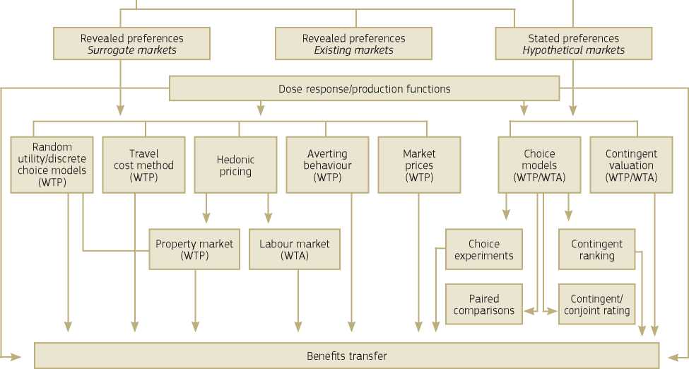
Source: Pearce, Atkinson, and Mourato (2006).
The monetary measure of a change in an individual’s well-being due to a change in environmental quality is called the total economic value of the change. The total economic value of a resource can be divided into use values and non-use values; i.e. total economic value = use values + non-use values.
- Use value. This refers to the social value people have from actually using a good or potentially using it in the future (e.g. recreational activities, productive activities such as agriculture and forestry, etc.), as well the benefits derived from the goods and services provided by the ecosystem that are used indirectly by an economic agent (e.g. the purification of drinking water filtered by the soil). They are called, respectively, ‘actual’, ‘option’ and ‘indirect’ values.
In this context, uncertainty stems from a combination of the individual’s uncertainty about future demand for the resource and uncertainty about its future availability.
- Non-use value. Each individual could be assumed to place a value not only on the well-being produced by the good’s existence per se on himself/herself (existence value), but also on the well-being caused to other individuals by the availability of that good, either in the same generation (altruist value) or future generations (bequest value). Non-use values are less tangible than use values since they do not refer to a physical consumption of goods and services.
Values are directly linked to the ecological services produced by the ecosystems, which support them. A reduction in the provision of ecological services (by a pollution, for example) is likely to depreciate the values expressed by people on environmental quality with, as a final result, a decrease in social benefits associated with it. It is important to understand that economic value does not measure environmental quality per se; rather it reflects people’s preferences for that quality. Evaluation is ‘anthropocentric’ in that it relates to preferences held by people.
Non-Use
Use Value
Total Economic Value (TEV)
Value
|
Direct use |
Option | ||
Direct benefits from use of primary goods
Option for future use (direct or indirect) of goods & services
\
secondary goods & services (including non consumptive use) m\
Philantropic value Bequest & Altruist
Existence value
Provisioning services:
• Timber & Fuel wood
• Food/fodder & other forest products (latex)
• Bioprospecting: bio-chemicals, medicines
• Fresh water Cultural services:
• Recreation
• Tourism
• Education/science
Provisioning services:
• Fresh water
• Bioprospecting Regulating services:
• Carbon storage
• Air quality & water purification
• Erosion control
• Natural hazards management Cultural services:
• Scenery, recreation Supporting services:
• Soil quality
Bequest value (value for future generations) Altruist value (value for others)
Provisioning services:
• Fresh water Regulating services:
• Carbon storage
• Air quality Cultural services:
• Scenery / landscape
• Recreation
• Education / science Supporting services:
• Soil quality
Value of existence without use/ consumption of goods or services
Cultural services:
• Scenery / landscape
• Community identity / integrity
• Spiritual value Wildlife/biodiversity
Source: EU (2013) The Economic benefits of the Natura 2000 Network
The dose-response technique aims to establish a relationship between environmental impacts (the response) and physical environmental impacts such as pollution (the dose). The technique is used when the dose-response relationship between the cause of environmental damage, such as air or water pollution, and the impacts, for example morbidity due to air pollution or water contamination by chemical products, is well known. The technique takes natural science information on the physical effects of pollution and uses this in an economic model of evaluation. The economic evaluation will be performed by estimation, through a production or a utility function of the profit variations of businesses or the revenue gains or losses of individuals.
The two steps of the method are:
• the calculation of the pollutant dose and receptor function, and
• the economic evaluation by the choice of an economic model.
To assess the monetary gain or loss of benefits due to the variation in environmental quality requires the analysis of biological and physical processes, their interactions with economic agents' decisions (consumer or producer) and the final effect on welfare.
The major fields of application of the methodology are the evaluation of losses (in crops, for example) due to pollution, the pollution effects on ecosystems, vegetation and soil erosion, and the impacts of urban air pollution on health, materials and buildings. The approach cannot estimate the non-use value.
Different methods can be adopted to empirically estimate the WTP as a welfare measure. Three main methodological categories (i.e. revealed preference methods; stated preference methods; benefit transfer method) are discussed below, which are well established and consolidated in both the theory and practice of CBA. That said, research in this area is ongoing and novel approaches are being developed369. The methodology is still evolving and existing valuations are not robust enough yet for use in value transfer for CBA, but due consideration will be given to future developments.
This approach implies that the valuation of non-market impacts is based on the observation of the actual behaviour and, especially, on the purchases made in actual markets. Consequently, the focus is on real choices and implied willingness to pay. The strength of these approaches is that they are based on actual decisions made by individuals. The main weakness is the difficulty of testing the behavioural assumptions upon which the methods rely. The main specific methods are:
• hedonic pricing/wage method;
• travel cost method;
• averting or defensive behaviour method.
The focus of this method is in the observation of behaviour in markets for goods related to the ones the analyst is evaluating. The starting point is the fact that the prices of many market goods are functions of a bundle of characteristics. For example, the price of a washing machine usually depends on the variety of washing programmes, its energy efficiency and its reliability. Through statistical techniques the method tries to isolate the implicit price of each of these characteristics.
In non-market evaluation the method uses two types of markets:
• property market,
• labour market.
With regard to the property market, houses can be described through their structural characteristics (e.g. number of rooms), locational characteristics (e.g. proximity to schools), neighbourhood characteristics (e.g. crime rates) and environmental characteristics (e.g. road traffic noise). The hedonic pricing method should identify the contribution of each significant determinant of house prices in order to estimate the marginal willingness to pay for each characteristic. Hedonic studies of the property market have been used to identify the value of non-market goods, such as traffic noise, aircraft noise, air pollution, water quality and proximity to landfill sites. A house near an airport, for example, will be purchased at a lower price than a house located in a quiet area, everything else being equal. The difference in values can be viewed as the value attached to noise. The creation of an urban park in a disused industrial area or the urban improvement of a neighbourhood result in an increase in the market value of the properties in the project area. The total increase of the estate value is a good proxy of the socioeconomic benefit of the project.
In the labour markets, the observation of wage differentials between jobs with different exposure to physical risk is used in order to estimate the value of avoiding risk of death or injury.
Specific problems with this approach could be a lack of information on household data and the fact that market characteristics tend to move in tandem; it is often hard to ‘tease out' the independent effect of a single characteristic. For further information on how to conduct the hedonic price analysis with one of the methods, see the relevant bibliography.
The project concerns a small neighbourhood that includes residential and commercial areas and services in a medium-sized town. The socioeconomic benefit of the intervention can be valued by the expected increase in the real estate prices of buildings in the neighbourhood due to the improved urban functions. This is the hedonic price, regardless of whether the properties will be actually traded.
The used surfaces of the buildings amount to 535,500 square meters. Taking into account the different destinations of use, the average price on the real estate market in the neighbourhood is currently EUR 1,110/m2. Looking at the real estate market in other districts of the same city and at other cities with similar characteristics, analysts have concluded that the average price in the areas already rehabilitated, which is obviously higher, may be set at EUR 1,385/m2. The potential increase in the price of the real estate is therefore 1,385 - 1,110 = EUR 275/m2. Therefore the total benefit of the project amounts to 535,500 x 275 = EUR 147,262,500.
Given that the positive impact of the project on the neighbourhood does not develop in a single moment, but will take some time, the total benefit, as calculated above, should be appropriately divided into a proper number of years of the time horizon of the analysis. For example, if the urban rehabilitation works take two years, and assuming that the effects will develop in the next three years, it will be appropriate to allocate three equal inputs, each of EUR 49,087,500, over the third, fourth and fifth years of the analysis horizon.
Source: Authors
The travel cost approach seeks to put a value on individuals WTP for access to environmental resources, for instance outdoor recreation areas, by looking at the costs incurred to access them.
The basis of the method is the observation that travel and outdoor recreation areas are complements such that the value of the recreation areas can be measured with reference to values expressed in the markets for trips to those areas. For zones located too far from the area the number of visits is zero because the cost of the trip exceeds the benefit derived from the trip. Therefore it is important to know the following:
• the number of trips to the outdoor recreation areas over a given time period;
• the costs of the trips to these from different zones, split into different components:
- the monetary costs; including travel costs, admission price (if relevant), on-site expenditures, expenditure on capital equipment necessary for consumption;
- the time spent travelling and its value.
Specific problems with this approach are related to ‘multiple purpose trips'; because many trips have more than one destination, it is difficult to identify which part of the total travel cost is related to one specific destination. Another problem is that the travel cost method allows an estimation of the WTP for the entire site, rather than a specific feature of it and this may make it problematic to estimate the value of a change in one attribute of a multi-dimensional good.
Since only the benefits of the direct consumption of the environmental services are considered in this approach, non-use (existence, altruist and bequest) values cannot be considered.
Mendes and Proenęa (2005) provided an example of empirical estimation on the recreation value of ecosystems. They proved that the Portuguese Peneda-Gere National Park is able to produce a significant social benefit, which could justify the allocation of more public resources to eco-tourism activities.
Starting from the generic economic definition that the marginal recreation value of an ecosystem is equal to the amount visitors would pay to enjoy recreation and leisure activities, the authors estimated the relationship between the costs incurred by travellers to a site and the number of trips taken. During the 1994 summer peak-period months, questionnaires were distributed to Portuguese citizens’ over 18 years old who were visiting the park at that time for visits equal or longer than 24 hours. Information was gathered about the number of days of stay, income, the geographical origin, the cost of the trip, transportation mode and various demographic characteristics. The demand of recreation per trip has been modelled as a function of the cost incurred, available income and individual characteristics (plus an independent error term). The consumer surplus of the representative visitor per each average day of stay has been derived by integrating the recreation demand function over the relevant cost change. From here, the value of the willingness to pay has been estimated through the formula proposed by Grogger and Carson (1991) and Englin and Shonkwiler (1995).
Results show one recreation day was valued EUR 124 (2005 prices) for the average representative visitor of the sample. Considered that approximately 12,000 visitors camp in the park every year, this generates a benefit of EUR 1,488,000.
Source: Florio (2014)
The main assumption of the averting evaluation method is that individuals can insulate themselves from a non-market good by adopting more costly behaviours to avoid it. The cost these behaviours require can be represented by extra time or by the restrictions they impose on what individuals would otherwise wish to do.
Another way to avoid exposure to a specific non-market good is the purchase of a market good to ‘defend' the consumer from the ‘bad' (defensive expenditures). The value of each of these purchases can be considered the implicit price for the non-market good that individuals want to avoid.
An example could be the installation of double-glazed windows to decrease exposure to road traffic noise. Double-glazing is a market good that can be seen as a substitute for a non-market good (absence of road traffic noise) and so the cost of purchasing it can be considered as the price of the non-market good. Specific problems with these approaches could be:
• defensive expenditures often represent a partial estimate of the value of the non-market good individuals want to avoid;
• many averting behaviours or defensive expenditures are related to joint products (e.g. heating and insulation from noise);
• individuals or businesses may undertake more than one form of averting behaviour in response to any environmental change.
Stated preference approaches are survey-based and elicit people's intended future behaviour in the markets. Through an appropriately designed questionnaire, a hypothetical market is described where the good in question can be traded. A random sample of people is then asked to express their maximum willingness to pay for (or willingness to accept) a supposed change in the good's provision level.
The main strength of the methods based on this approach is represented by the flexibility they can assure. Indeed, they allow the evaluation of almost all non-market goods, both from an ex ante and from an ex post point of view. Moreover, this methodology is able to capture all types of benefits from a non-market good or service, including the so-called non-use values.
The main specific methods are:
• contingent valuation method, • choice modelling method.
The aim of the contingent valuation method is to elicit individual preferences, in monetary terms, for changes in the quantity or quality of a non-market good or service.
The key element in any contingent valuation study is a properly designed questionnaire. The questionnaire aims to determine individuals' estimates of how much having or avoiding the change in question is worth to them. In order to conduct a contingent valuation it is worthwhile:
• investigating the attitudes and behaviour related to the goods to be valued in preparation for answering the valuation question and in order to reveal the most important underlying factors driving respondents' attitude towards the public good;
• presenting respondents with a contingent scenario that provides a description of the commodity and the terms under which it is to be hypothetically offered. The final questions should aim to determine how much they would value the good if confronted with the opportunity to obtain it under the specified terms and conditions;
• asking questions about the socioeconomic and demographic characteristics of the respondents in order to check the extent to which the survey sample is representative of the population involved;
• asking respondents whether they would be willing to pay a specified amount for the good; if the answer is affirmative, the interviewer would repeat the questions by slightly increasing the price until the respondent expresses an unwillingness to pay the amount specified.
At the end of the survey process, analysts use appropriate econometric techniques to derive welfare measures, such as mean or median willingness to pay and also to identify the most important determinants of willingness to pay. With regard to the statistical indicators to be used, the median could be the best predictor of what the majority of people would actually be willing to pay because, unlike the mean, it does not give much weight to outliers.
Problems with contingent valuation are associated with the probability that respondents do not fully understand the scenario or what the good in question is, or that they are not willing to attach a monetary value to certain goods (such as, for example, the value of a human life). Additionally, Carson and Groves (2007) point out that an increase in the provision of a public good for which only voluntary contribution is asked, is generally overvalued: this is because respondents have an incentive to free-ride in order to increase the chances of provision of the desired good without having to pay for it.
Choice modelling (CM) is a survey-based method for modelling preferences for goods, when goods are described in terms of their attributes and of the level of these attributes. Respondents have various alternative descriptions of a good, differentiated by their attributes and levels, and are requested to rank the alternatives, to rate them or to choose their preferred option. By including price/cost as one of the attributes of the good, willingness to pay can be directly recovered from people's rankings, ratings or choices. Also, in this case, the method allows the measurement of non-use values.
The main variants proposed in specialist literature are described in the following table.
|
Main variants of the CM method |
Tasks |
|
Choice experiments |
Choose between two or more alternatives (where one is the status quo) |
|
Contingent ranking |
Rank a series of alternatives |
|
Contingent rating |
Score alternative scenarios on a scale of 1 to 10 |
|
Paired comparison |
Score pairs of scenarios on a similar scale |
The main strengths of the method are:
• the capacity to deal with situations where changes are multi-dimensional, thanks to its ability to separately identify the value of the specific attributes of a good;
• the possibility for respondents to use multiple choices (for example variants in choice experiments), to express their preference for a valued good over a range of payment amounts;
• by relying on ratings, rankings and choices, and deriving indirectly from the willingness to pay of respondents, the method overcomes some problems associated with the contingent valuation method.
The main weaknesses are:
• the difficulties respondents experience in dealing with multiple complex choices or rankings;
• the inefficiency in deriving values for a sequence of elements implemented by a policy or project. For these types of evaluations contingent methods should be preferred;
• the willingness-to-pay estimate is sensitive to study design. For example, the choice of attributes and levels to present to the respondents and the way in which choices are relayed to respondents (use of photographs, text description, etc.) may impact on the values of estimates.
Developments in policy behaviour have stressed the relevance of the so-called benefit transfer approach (or method) in the appraisal of non-market goods, specifically environmental goods and services (Pearce, Atkinson and Mourato, 2006). This method consists of taking a unit value for a non-market good estimated in an original study and using this estimate, after some adjustments, to value benefits (or costs) that arise when a policy or project is implemented elsewhere.
The benefit transfer method can be defined as the use of a good estimate in one site, the ‘study site' as a proxy for values of the same good in another site, the ‘policy site'. For example, the provision of a non-market good at a policy site could refer to a lake at a particular geographical location. If sufficient data is not available for that country, analysts can use values for similar conditions in data-rich countries.
The interest shown in this approach is due to the opportunity to reduce the need for costly and time-consuming original studies of non-market goods values. Moreover, benefit transfer could be used to assess whether or not a more in-depth analysis is worthwhile.
Clearly, the main obstacle in using this approach is that benefit transfer can give rise to seriously biased estimates, though obviously judgement and insight are required for all the basic steps entailed in undertaking a benefit transfer exercise. For example, information needs to be obtained on baseline environmental quality, changes and relevant socioeconomic data.
Benefit transfer is usually performed in three steps:
• compilation of the existing literature on the subject under investigation (recreational activity, human health, air and water pollution, etc.);
• assessment of the selected studies for their comparability (similarity of the environmental services or benefits valued, difference in revenue, education, age and other socioeconomic characteristics which can affect the evaluation);
• calculation of values and their transfer in the new context of evaluation.
The most crucial stage is where existing estimates or models are selected and the estimated effects are obtained for the policy site. In addition, the population at the relevant policy site must be determined.
Adjustments are usually advisable in order to reflect differences at the original study sites and the new policy sites. The analyst may choose from three main types of adjustment of increasing sophistication:
• unadjusted willingness-to-pay transfer. This procedure implies a simple ‘borrowing' of the estimates made in the study site and the use of those estimates in the policy site, with an obvious advantage in terms of simplicity;
• willingness-to-pay transfer with adjustment (value transfer). It could be useful to modify the values from the study site data to reflect the difference in a particular variable that characterises the sites; for example, the values can be adjusted through multiplication using the ratio between the income level of the study case and the income level of the policy case;
• willingness-to-pay function transfer. A more sophisticated approach is to transfer the benefit or value function from the study site to the policy site. Thus, if it is known that the willingness to pay for a good at the study site is a function of, first, a range of physical features on the site, second, of its use, and third, of a set of socioeconomic characteristics of the population at the site, then this information itself can be used as part of the transfer process.
The benefit transfer method was used by the European Commission to value the willingness to pay (WTP) for the construction of nine waste water treatment plants in eight municipalities of Ria de Vigo (Spain). Implemented between 1995 and 2000, the infrastructure project was addressed to improve the quality of life of beneficiaries, thanks to the possibility of enjoying cleaner water and more numerous bathing beaches. The reference studies to estimate the WTP for the waste water treatment of Ria de Vigo were selected from a database of 40 cases (US Environmental Protection Agency 2000a, 2000b, 2000c; Kallstram 2010) on the basis of two criteria: the type of project and the socioeconomic context of the country. With regard to the former, only waste water treatment projects that were effective in improving the quality of the water basin and in which the sewerage system was already in place, as in the municipalities of Ria de Vigo, were selected. For the selection of the most similar socioeconomic context, evaluators considered projects in those countries falling under the classification of very high and highly developed countries, according to the UNDP Human Development Index 2011. These first two steps enabled the identification of 28 projects in different countries of the world. The WTP values that referred to each of the 28 selected projects were divided by the national per capita GDP, which was taken as a proxy of the differences in the per capita income.
The WTP for the project in Ria de Vigo was then calculated as the average WTP for the 28 projects considered, weighted by GDP, and in turn weighted by Spanish per capita GDP. This amounted to EUR 88.11 per household (2011 prices). The described methodology implicitly assumes the income elasticity of WTP as being equal to 1, meaning that the ratio of WTP valued in each of the 28 reference countries and in Ria de Vigo is equivalent to the ratio of per capita GDP at the different sites.
Source: European Commission (2012)
For all types of adjustments, the quality of the original study is of paramount importance for the validity of the method.
Some databases have been set up to facilitate benefit transfer. This is the case with the EVRI database370 developed by Environment Canada and the US Environment Protection Agency. More than 700 studies are currently available in the database, but only a minority are of European origin and this fact reduces the usability of the database in a European context. GEVAD is an online European database, which was co-funded by the European Social Fund and Greek government resources. The aim of the project was to create a free online environmental valuation database, by gathering a critical mass of European valuation studies. About 1,400 studies were reviewed, focusing on the ones that were spatially more relevant to Europe. Emphasis was also placed on the most recent research results. So far, more than 310 studies have been included in the GEVAD database. These studies are classified according to the environmental asset, good or service, which is valued (e.g. amenities, water and air quality, land contamination, etc.), the valuation method used, the main author and the country of the ‘study site'.371
As explained in the main text, the WTP for mortality risk reductions is normally expressed in terms of the value of statistical life (VOSL). The following table has a variety of estimates on the VOSL, mostly for the UK. There is some unease about using the value of statistical life in contexts where remaining years may be few for the affected individuals and this has led to the use of ‘life year’ valuations derived from VOSL. For example, the concern is that estimates of VOSL from studies of workplace accidents (which tend to affect healthy, middle-aged adults) and road accidents (which tend to affect median-aged individuals) are ‘too high’ when transferred to environmental contexts where mortality-related air pollution impacts tend to mostly affect the very elderly or those with serious respiratory problems.
|
Study |
Type of study |
Risk Context |
VOSL $Million (year prices) |
|
Markandya et al. 2004 |
Contingent valuation |
Context-free reduction in mortality risk between ages of 70 and 80 |
1.2-2.8 0.7-0.8 0.9-1.9 (2002)3 |
|
Chilton et al. 2004 |
Contingent valuation |
Mortality impacts from air pollution |
0.3-1.5 (2002)3, 4 |
|
Chilton et al. 2002 |
Contingent valuation |
Roads (R), Rail (Ra) |
Ratios: Ra/R=1.0036 |
|
Beattie et al.1998 |
Contingent valuation |
Roads (R) and domestic fires (F) |
5.73 |
|
Carthy et al. 1999 |
Contingent valuation/standard gamble |
Roads |
1.4-2.3 (2002)3, 5 |
|
Siebert and Wie 1994 |
Wage risk |
Occupational risk |
13.5 (2002)3 |
|
Elliott and Sandy 1996 |
Wage risk |
Occupational risk |
1996: 1.2 (2000)3 |
|
Arabsheibani and Marin 2000 |
Wage risk |
Occupational risk |
1994: 10.7 (2000)3 |
Note: 1: median of the studies reviewed; 2: range varies with risk reduction level; lower VOSLs for larger risk reductions.
3: Gross national income in GBP converted to USD using purchasing power parity rates per capita ratio between UK and US. Range reflects different risk reductions. 4: based on WTP to extend life by one month assuming 40 years of remaining life. 5: based on trimmed means. 6: this study sought respondents’ relative valuations of a risk relative to a risk of death from a road accident. Numbers reported here are for the 2000 sample rather than the 1998 sample. Between the two sample periods there was a major rail crash in London.
Source: Pearce, Atkinson and Mourato (2006).
This annex explains how to use the main project performance indicators for CBA analysis: net present value, internal rate of return (IRR) and the benefit-cost (B/C) ratio.
The net present value of a project is the sum of the discounted net flows of a project. The net present value is a very concise performance indicator of an investment project: it represents the present amount of the net benefits (i.e. benefits less costs) flow generated by the investment expressed in one single value with the same unit of measurement used in the accounting tables.
It is important to note that the balance of costs and benefits in the early years of a project is usually negative and it only becomes positive after some years. As at decreases with time, negative values in the early years are weighted more than the positive ones occurring in the later years of a project's life. The value of the discount rate and the choice of the time horizon are crucial for the determination of the net present value of a project.
Net present value is a very simple and precise performance indicator. A positive net present value, net present value>0, means that the project generates a net benefit (because the sum of the weighted flows of costs and benefits is positive) and it is generally desirable either in financial terms or in economic terms. When different options are considered, the ranking of the net present values of the alternatives indicates the best one. For instance in Figure VII.1, project 1 is more desirable than project 2 because it shows a higher net present value for all the discount rates (i) applied.
There are cases in which the net present value of one alternative is not greater than the other or for every i value. This is due to a phenomenon referred to as ‘switching'. Switching occurs when the net present value curves of two projects intersect one another, as in Figure VII.2. With a discount rate above x, project 1 has a higher net present value; with a discount rate below x, project 2 will perform better. In order to select the best option, the definition of the discount rate is crucial for the selection of the best option (and IRR cannot be used as a decision rule).
Figure VII.1 Project ranking by net present values Figure VII.2 A case of switching
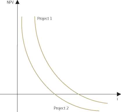
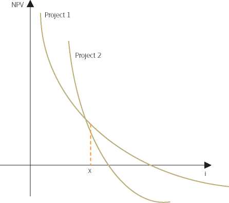
The internal rate of return (IRR) is defined as the discount rate that zeroes out the net present value of flows of costs and benefits of an investment. The IRR is an indicator of the relative efficiency of an investment, and should be used with caution. The relationship between net present value and IRR is shown in the graph below.
Figure VII.3 The internal rate of return Figure VIII.4 Multiple IRRs
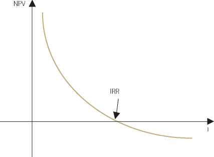
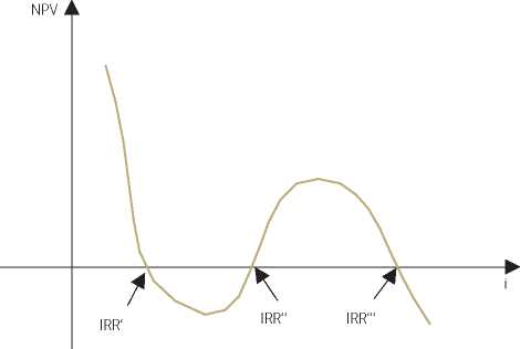
If the “sign” of the net benefits changes in the different years of the project's lifespan (for example: - + - + etc.), there may be multiple IRRs for a single project. In these cases the IRR decision rule is impossible to implement. Examples of this type of project are mines and nuclear power plants, where there is usually a large cash outflow at the end of the project because of decommissioning costs.
As IRR rankings can be misleading, and given that the informational requirements for computing a proper net present value and IRR are the same except for the discount rate, it is always worth calculating the net present value of a project. There are many reasons in favour of the net present value decision rule (see Ley, 2007).
The IRR contains no useful information about the overall economic value of a project. This can be illustrated by graphing the net present value as a function of the discount rate (r). Consider Figure VII.5, which displays the net present value schedule for two alternative projects. Project A has a substantially higher net present value for any discount rate in the economically relevant range (i.e. for any r less than 30 %), yet it crosses the axis to the left of project B, and consequently has a lower IRR - i.e. IRRA = 40 % < IRRB = 70 %.
Figure VII.5 IRR and net present value of two mutually exclusive alternatives
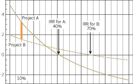
0 0.2 0.4 0.6 0.8 1
Discount Rate
Source: Ley (2007).
Since welfare depends on net present value, not IRR, it is apparent that project A dominates B. For instance net present value A(r) exceeds net present value B(r) by about USD 1.6 million for a discount rate in the region of 10 %.
Other shortcomings of the internal rate of return are:
• the sensitivity to economic life: when projects with different economic lives are to be compared, the IRR approach inflates the deliverability of a short-life project because IRR is a function both of the time period and of the size of capital outlay;
• the sensitivity to the timing of benefits: when there are projects that fail to yield benefits for many years, the IRR tends to be lower compared to projects with a fairly even distribution of benefits over time, even though the net present value of the former may be higher;
• the IRR indicator cannot deal with cases in which time-varying discount rates are used. In these cases, the net present value rule allows discount rate changes to be incorporated easily into the calculation.
One advantage of the IRR (under reasonable assumptions) is that it is a pure number and this makes it easier to compare projects that are similar, apart from their size.
The benefit-cost ratio is the present value of project benefits divided by the present value of project costs. If B/C >1, the project is suitable because the benefits, measured by the present value of the total inflows, are greater than the costs, measured by the present value of the total outflows.
Like the IRR, this ratio is independent of the size of the investment, but in contrast to IRR it does not generate ambiguous cases and for this reason it can complement the net present value in ranking projects where budget constraints apply. In these cases, the B/C ratio can be used to assess a project's efficiency.
The main problems with this indicator are:
• it is sensitive to the classification of the project effects as benefits rather than costs. It is relatively common to have project effects that can be treated both as benefits and as cost reductions and vice versa. Since the benefit-cost ratio rewards projects with low costs, considering a positive effect as a cost-reduction rather than a benefit would only result in an artificial improvement of the indicator;
• it is not appropriate for mutually exclusive projects. Being a ratio, the indicator does not consider the total amount of net benefits and therefore the ranking can reward more projects that contribute less to the overall increase in public welfare.
The appropriate case for using the B/C ratio is under capital budget constraints. The following table provides an example of project ranking given a budget constraint of 100.
Table VII.1 Benefit-cost ratio under budget constraints
|
PV (O) |
PV (I) |
Net present value |
PV(I) / PV(O) | |
|
Project A |
100 |
200 |
100 |
2.0 |
|
Project B |
50 |
110 |
60 |
2.2 |
|
Project C |
50 |
120 |
70 |
2.4 |
Looking at net present value, the preferred project is A and the ranking is A, C, B. But looking at the ratios between PV(I) and PV(O), C is the favourite project. Since the budget constraint is 100 and the PV(O) of project C is 50, project B, the second in the ranking, could also be undertaken. The resulting net present value (net present value(B)+net present value(C)) is 130, which is higher than the net present value of project A.
Forecasting the future value of variables, an exercise needed in the ex ante project analysis, involves an unavoidable degree of uncertainty. Uncertainty is inherent both in the factors internal to the CBA model (as, for example, the value of time savings, the hedonic pricing in an urban area, the timing of the completion of the investment, the value of the CO2 added or avoided, etc.) and in the factors external to the CBA model (for example, the future prices of inputs and outputs of the project, the actual cost of the investment, the actual number of the future users of the service held by a project infrastructure, etc.). In the former case, the uncertainty arises from the analyst estimate of the most appropriate values to set for the model parameters, regardless of the predictions on the running of the project; in the latter case, the uncertainty relates to the expected values of input and output variables that will materialise over the life of the project.
The uncertainty of the variables results in an uncertainty in the results of the cost-benefit analysis. In other words the actual values of the performance parameters may be different, even very different, from those calculated in the ex ante exercise: the project could show a contribution to a social welfare minor compared to what is expected, and even a default.
Risk assessment is aimed at evaluating this uncertainty and moving towards the adoption of measures for risk prevention and mitigation of adverse effects. As stated in Chapter 2, risk assessment, in the broad sense, requires:
• sensitivity analysis,
• qualitative risk analysis,
• probabilistic risk analysis underpinned on the probability distribution of critical variables372,
• assessment of acceptable levels of risk,
• risk prevention.
The overall risk assessment methodology is set out in section 2.10. The next sections of this annex deal with the probabilistic risk analysis and give additional information on risk assessment and mitigation.
Once the critical variables have been identified, then, in order to determine the nature of their uncertainty, probability distributions should be defined for each variable. A distribution describes the likelihood of occurrence of values of a given variable within a range of possible values around the best estimate, used as the base case.
There are two main categories of probability distribution in literature:
• ‘discrete probability distribution', when only a finite number of values can occur;
• ‘continuous probability distribution', when any value within the range can occur.
If a variable can assume a set of discrete values, each of them associated with a probability, then it is defined as discrete distribution. This kind of distribution may be used when the analyst has enough information about the variable to be studied, so as to believe that it can assume only some specific values.
Figure VIII. 1 Discrete distribution
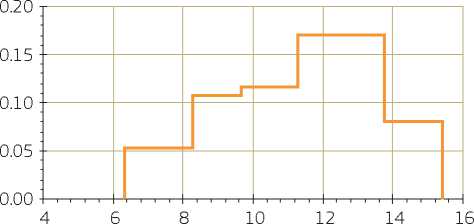
Gaussian (or Normal) distribution is perhaps the most important and the most frequently used probability distribution. This distribution (see Figure VIII. 2) is completely defined by two parameters:
• the mean (p)
• the standard deviation (a).
The degree of dispersion of the possible values around the mean is measured by the standard deviation373'
Figure VIII. 2 Gaussian distribution
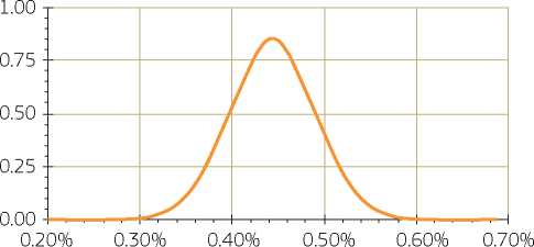
Normal distributions occur in many different situations374. When there is reason to suspect the presence of a large number of small effects acting additively and independently, it is reasonable to assume that observations will be normally distributed.
Triangular or three-point distributions are often used when there is no detailed information on the variable's past behaviour. This simple distribution is completely described by a ‘high value', a ‘low value' and the ‘best-guess value', which, respectively, provide the maximum, the minimum and the modal values of the probability distribution.
Triangular distribution is typically used as a subjective description of a population for which there is only limited sample data, and especially in cases where the relationship between variables is known but data is scarce (possibly because of the high cost of collection). The precise analytical and graphical specification of a triangular distribution varies a great deal, depending on the weight given to the modal value in relation to the extreme point values.
Figure VIII. 3 Symmetric and asymmetric triangular distributions
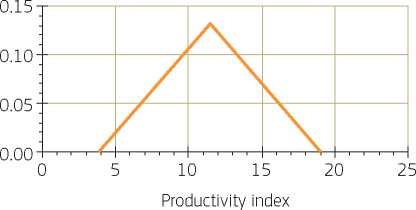
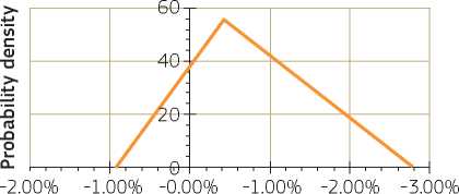
Accrual/year of real wage growth
The diagrams in Figure VIII. 3 show two types of triangular distributions.
• The first one is symmetric, with the high value as likely as the low ones and with the same range between the modal value and the low value, and between the modal value and the high value.
• The second one is asymmetric, with the high value more likely than the low ones, and with a larger range between the modal value and the high value than the range between the modal value and the low value (or vice-versa).
If there is no reason to believe that within a range a given value is more likely to materialise than others, the distribution obtained is called ‘uniform', i.e. a distribution for which all intervals of the same length on the distribution's support are equally probable.
The question of where to look for relevant distributions arises. As set out in section 2.1.3, the probability distribution for each variable may be derived from different sources, such as experimental data, distributions found in the literature for similar cases and consultations with experts. One possible approach is ‘reference forecasting', i.e. taking an ‘outside view' of the project by placing it in a statistical distribution of outcomes from a class of similar projects. It requires the following three steps:
• the identification of a relevant reference class of past projects, sufficiently broad to be statistically meaningful without becoming too generic;
• the determination of a probability distribution of the outcomes for the selected reference class of project;
• a comparison of the specific project with the reference class distribution and a derivation of the expected outcome.
According to Flyvberg (2005) ‘The comparative advantage of the outside view is most pronounced for non-routine projects. It is in planning such new efforts that the biases toward optimism and strategic misrepresentation are likely to be largest.'
Having established the probability distributions for the critical variables, it is possible to proceed with the calculation of the probability distribution of the project's net present value (or the IRR or the B/C ratio). The following table shows a simple calculation procedure that uses a tree development of the independent variables. In the sample reported in the table, given the underlying assumptions, there is 95 % probability that the net present value is positive.
Table VIII.1 Probability calculation for net present value conditional to the distribution of critical variables in millions EUR
|
Investment Value |
Critical variables |
Result | ||||
|
Other costs |
Benefit |
Net present value | ||||
|
Value |
Probability |
Value |
Probability |
Value |
Probability | |
|
-56.0 |
-13.0 |
0.20 |
74.0 |
0.15 |
5.0 |
0.03 |
|
77.7 |
0.30 |
8.7 |
0.06 | |||
|
81.6 |
0.40 |
12.6 |
0.08 | |||
|
85.7 |
0.15 |
16.7 |
0.03 | |||
|
-15.6 |
0.50 |
74.0 |
0.15 |
2.4 |
0.08 | |
|
77.7 |
0.30 |
T-1 ID |
0.15 | |||
|
81.6 |
0.40 |
10.0 |
0.20 | |||
|
85.7 |
0.15 |
14.1 |
0.08 | |||
|
-18.7 |
0.30 |
74.0 |
0.15 |
-0.7 |
0.05 | |
|
77.7 |
0.30 |
3.0 |
0.09 | |||
|
81.6 |
0.40 |
6.9 |
0.12 | |||
|
85.7 |
0.15 |
10.9 |
0.05 | |||
The more general approach to the calculation of the conditional probability of project performance is the Monte Carlo method (already presented in section 2.10. See also references in the bibliography). In a nutshell, the repeated extraction of a random set of values for the critical variables, taken in their respective intervals, allow the calculation of the performance indices for the project (IRR or net present value) that result from each set of values extracted. By repeating this procedure for a large enough number of extractions one can obtain the probability distributions of the IRR or net present value.
Often the net present values and IRRs reported in project appraisal reports refer to best or baseline estimates, perhaps meaning ‘most likely' values (or mode). However, the criterion for project acceptability should be that of the expected value (or mean) of such indicators, calculated from the underlying probability distributions.
For instance, if a project has an ERR of 10 % but also the probability risk analysis tells us that the ERR has a value between 4 and 10 with a probability of 70 % and a value between 10 and 13 with a probability of 30 %, then the expected value of ERR for that project is only 8.35 % (average (4,10)*0.7 + average(10,13)*0.3).
Whether a more thorough risk assessment is deemed necessary, risk scores or indices, based on processing the results of Monte Carlo simulations in a more or less sophisticated way, may be found in the literature.
In conclusion, the procedure described in this annex allows for the selection of projects not only on the basis of the best estimate, but also based on the risk associated with it, simply by weighting the performance with the risk. The expected performance, and not the modal one, is the value that should be reported in the application form for major projects requiring EU assistance, whenever a probabilistic risk analysis is carried out. In order to evaluate the result, one very important aspect is the compromise to be made between high-risk projects with high social benefits on the one hand, and low-risk projects with low social benefits on the other.
Generally, a neutral attitude towards risks is recommended because the public sector might be able to pool the risks of a large number of projects. In such cases, the expected value of the ERR could summarise the risk assessment. In some cases, however, the evaluator or the proposer can deviate from neutrality and prefer to risk more or less for the expected rate of return; there must, however, be a clear justification of this choice.
When individuals attach greater importance to the possibility of losing a sum of money than to the possibility of gaining the same sum, with a 50 % probability of each outcome occurring, there is ‘risk averse behaviour'.
Risk aversion follows from the proposition that the utility derived from wealth rises as wealth rises, but at a decreasing rate. This, in turn, comes from the theory of diminishing marginal utility of wealth. In microeconomic theory, it is generally assumed that the utility of the marginal quantity of a good is lower than the utility of the same quantity obtained before the marginal one.
Figure VIII.4 Relationship between utility and wealth for a risk averse society
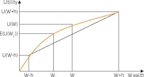
In Figure VIII.4, the utilities associated with the wealth levels W+h, W and W-h are indicated on the vertical axis. The expected utility of wealth for the society if the investment is realised is indicated on the vertical axis as well (E(U(W1)). Since there is a 50 % chance of gaining and a 50 % chance of losing, the value is exactly in the middle between (U(W+h) and U(W-h): E(U(W1)=0.5U(W-h) + 0.5U(W+h). But, because of the shape of the utility function (deriving from diminishing marginal utility of wealth assumption), the expected utility of wealth E(U(W1)) will be lower than the utility associated with the initial level of wealth W, i.e. E(U(W1)) < U(W). Consequently, the risk averse decision-maker will decide to reject the project. However, for the public sector, risk neutrality is to be assumed in general for a risk pooling (and spreading) argument. Under risk neutrality, the expected value of the net present value (the mean of probabilities) replaces the baseline or modal estimate of the net present value as a performance indicator.
As mentioned in section 2.10, the measures of risk prevention and/or mitigation should be tailored to the specific project and its level of risk. In this regard, an extensive analysis of adverse events and their causes, as well as of their potential negative effects on the project running, could help to outline the more effective and appropriate actions of risk prevention (see section 2.10.2).
However, the investment projects show some common and general features of their risk profiles, which are discussed below.
The degree of risk is not always the same over the time horizon of the project realisation. It has been demonstrated by past experience and is generally accepted in literature that the riskiest phase of a project is the start-up. At that time most of the investment costs have been incurred but there may not yet be any feedback from an operational point of view. When the investment enters into the operations phase, the risk involved diminishes because the feedback becomes increasingly evident.
The above justifies why the importance of correlating the proposed prevention/mitigation measures with the project phases in which the adverse events might occur has been underlined in section 2.10.2.
Figure VIII.5 Levels of risks in different phases of a given infrastructure project
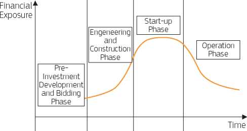
Moreover ‘there is a demonstrated, systematic tendency for project appraisers to be overly optimistic. To reduce this tendency, appraisers should make explicit, empirically based adjustments to the estimates of a project's costs, benefits and duration. It is recommended that these adjustments be based on data from past projects or similar projects elsewhere, and adjusted for the unique characteristics of the project in hand. In the absence of a more specific evidence base, departments are encouraged to collect data to inform future estimates of optimism, and in the meantime use the best available data.'375
According to Flyvbjerg and Cowi (2004) cost overruns and/or benefit shortfalls, i.e. optimism bias, are the results of a number of different factors:
• multi-actor decision-making and planning;
• non-standard technologies;
• long planning horizons and complex interfaces;
• changes in project scope and ambition;
• unplanned events.
As a result, cost overruns and benefit shortfalls lead to an inefficient allocation of resources, delays and further cost overruns and benefit shortfalls.
In addition to carrying out a full risk assessment, which represents a major step ahead in mitigating inaccuracy and bias, other measures recommended in order to reduce optimism are:
• better forecasting methods through the use of ‘reference class' forecasting;
• changed incentives in order to reward better projects;
• transparency and public control to improve accountability;
• involvement of private risk capital.
Table VIII.2 provides some examples of mitigation measures of identified risks extrapolated from the World Bank Project Appraisal Documents for different countries.
Table VIII.2 Risk mitigation measures
|
Country |
Project |
Risk |
Rating |
Risk mitigation measure |
|
Azerbaijan |
Power transmission |
Project implementation delays due to lack of local financing and poor project management |
S |
Local financing requirement minimised. Project Implementation Unit to be assisted by technical assistance for project management during implementation. |
|
Kyrgyzstan |
Water management improvement |
Counterpart funds are not available in timely manner |
N |
Project design minimises the need for counterpart funds, except for taxes. The Ministry of Economy and Finance has developed a satisfactory track record of support to ongoing International Development Association-funded irrigation projects. |
|
Russia |
Municipal heating |
Potential corruption may erode project benefits |
M |
Commercial and financial management systems for the project will provide more transparency and improve possibilities for adequate audit and control. |
|
Turkey |
Railway reconstruction |
Social resistance to change |
H |
Close cooperation between the government, General Directorate of State Railways Administration (TCDD) management and the trade unions; early definition of an appropriate social plan; expeditious payment of the severance benefits and assistance to staff. |
Source: World Bank Project Appraisal Documents. Note: Risk rating: H (high risk), S (substantial risk), M (modest risk), N (negligible or low risk).
While cost-benefit analysis is the most commonly used technique in appraising public investment and is the one required by the Funds' regulations for major projects, other kinds of project analysis exist and are used. In this section, the main features and fields of application of cost-effectiveness analysis (CEA) and multi-criteria analysis (MCA) are reviewed.
Cost-effectiveness analysis (CEA) is a comparison of alternative projects with a unique common effect, which may differ in magnitude. It aims to select the project that, for a given output level, minimises the net present value of costs or, alternatively, for a given cost, maximises the output level. CEA results are useful for those projects whose benefits are very difficult, if not impossible, to evaluate, while costs can be predicted more confidently. This methodology is often used in the economic evaluation of health-care programmes, but it can also be used to assess some education and environmental projects. For these examples, simple CEA ratios are used, such as the cost of education per student, the cost per unit of emission reduction, and so on. CEA is less helpful when a money value can be given to the benefits and not just to the costs.
Generally, CEA solves a problem of optimisation of resources that is usually presented in the following two forms:
• given a fixed budget and a number (n) of alternative projects, decision-makers aim to maximise the outcomes achievable, measured in terms of effectiveness (E);
• given a fixed level of E that must be achieved, decision-makers aim to minimise the cost (C).
While the measurement of costs is the same as in the financial analysis of CBA, the measurement of the effectiveness depends on the type of outcome chosen. Some examples of measures of effectiveness used in CEA are: number of life-years gained, days of disability avoided, test scores, etc. The box below briefly reviews the methodological approach of the CEA for project selection.
When the alternative projects are competitors and mutually exclusive, an incremental analysis is required in order to rank the projects and single out the one that is most cost-effective.
Generally cost-effectiveness analysis is pursued to test the null hypothesis that the mean cost-effectiveness of one project (a) is different from the mean cost-effectiveness of some competing intervention (b). It is calculated as the ratio (R):
R = (Ca - Cb) / (Ea - Eb) = AC / AE
defining the incremental cost per unit of additional outcome.
When a strategy is both more effective and less costly than the alternative (Ca - Cb < 0 and Ea - Eb > 0), it is said to ‘dominate’ the alternative: in this situation there is no need to calculate cost-effectiveness ratios, because the decision on the strategy to choose is obvious.
However, in most circumstances, the project under examination is contemporaneously more (or less) costly and more (or less) effective than the alternative(s) (Ca-Cb > 0 and Ea - Eb > 0 or, alternatively, Ca - Cb < 0 and Ea - Eb < 0). In this situation, the incremental cost-effectiveness ratios allow appraisers to rank the projects under examination and to identify, and then eliminate, cases of ‘extended dominance’. This can be defined as the state when a strategy is both less effective and more costly than a linear combination of two other strategies with which it is mutually exclusive. More operationally, extended dominance is where the incremental cost-effectiveness ratio for a given project is higher than that of the next more effective alternative.
In practice, CEA allows appraisers to exclude those project options that are not technically efficient (because of dominance), while for the remaining projects, the choice will depend on the size of the budget. The treatment with the lowest incremental cost-effectiveness ratio should be the first to be implemented and then other strategies should be added until the budget is exhausted.
There are also technical problems in aggregating outcomes that appear over different years, because it is not obvious what the specific discount factor should be (clearly neither the FDR nor the SDR apply to discounting numbers of students, patents or emissions).
In conclusion, cost-effectiveness analysis is a practical tool for project comparison when:
• the project produces only one output which is homogenous and easily measurable;
• this output is a crucial supply, entailing that action to secure it is essential;
• the aim of the major project is achieving the output at minimal cost;
• costs can be completely assessed for each alternative, i.e. hidden costs are more or less irrelevant;
• there are no relevant externalities;
• there is a wide evidence of benchmarks to verify that the chosen technology meets the minimum required cost performance criteria.
Multi-criteria analysis (MCA) is a family of algorithms used to select alternatives according to a set of different criteria and their relative ‘weights'. In contrast to CBA, which focuses on a unique criterion (the maximisation of social welfare), MCA is a tool for dealing with a set of different objectives that cannot be aggregated through shadow prices and welfare weights, as in standard CBA. MCA is appropriate for development programmes, pursuing simultaneously different policy objectives (e.g. equity, environmental sustainability, improved quality of life, etc.), rather than for the appraisal of a single investment project. There are many ways to design an MCA exercise. One possible approach is as follows:
• objectives should be expressed in measurable variables. They should not be redundant but could be alternative (the achievement of a bit more of one objective could partly preclude the achievement of the other);
• once the ‘objectives vector' has been determined, a technique should be found to aggregate information and to make a choice; the objectives should have assigned weights reflecting the relative importance given to them by the policy-maker;
• definition of the appraisal criteria; these criteria could refer to the priorities pursued by the different parties involved or they could refer to particular evaluation aspects;
• impact analysis: this activity involves describing, for each of the chosen criteria, the effects it produces. Results could be quantitative or qualitative;
• forecast of the effects of the intervention in terms of the selected criteria; from the results coming from the previous stage (both in qualitative and in quantitative terms), a score, or a normalised value, is assigned (this is the equivalent of ‘money' in CBA);
• identification of the typology of subjects involved in the intervention and the determination of respective preference functions (weights) accorded to different criteria;
• scores under each criterion are then aggregated (simply with a sum or with a non-linear formula) to give a numerical evaluation of the intervention; the result can then be compared with the result for other similar interventions.
The project examiner should then verify if:
• forecasts for non-monetary aspects have been quantified in a realistic way in the ex ante evaluation;
• there is in any case a CBA for the standard objectives (financial and economic analysis);
• the additional criteria under the MCA have a reasonable political weight, so as to determine significant changes in the financial and economic results.
When the benefits are not just non-monetary, but also physically not measurable, a qualitative analysis should still be conducted. A set of criteria relevant for the project appraisal (equity, environmental impact, equal opportunity) is collected in a matrix, together with the impacts (measured with scores or percentages) of the project on the relevant criteria. Another matrix should then assign weights to each relevant criterion. By multiplying scores and weights, the total impact of the project is obtained: this allows the selection of the best alternative.
If it is difficult to reflect the outcomes and/or costs of a project in measurable terms so that these measures can be aggregated in a CBA, it is recommendable to switch to a MCA with its multidimensional characteristics instead of forcing heterogeneous and diverse data into a quantitative economic calculus.
Belli, P., Anderson, J.R., Barnum, H.N., Dixon, J.A., Tan, J-P (2001), Economic Analysis of Investment Operations. Analytical Tools and Practical Applications, WBI, World Bank, Washington D.C.
Boardman, A.E., Greenberg, D.H., Vining, A.R. and Weimer, D.L. (2006), Cost-Benefit Analysis: Concepts and Practice, 3rd edition, Upper Saddle River, New Jersey: Pearson Prentice Hall.
CEPS, (2013), Assessing The Costs And Benefits Of Regulation. Study for the European Commission, Secretariat General, Brussels, 10 December 2013.
Dasgupta, P., Marglin, S. and Sen, A.K. (1972), Guidelines for project evaluation, New York: UNIDO.
European Investment Bank (2013), The Economic Appraisal of Investment Projects at the EIB. Available at: http://www.eib. org/infocentre/publications/all/economic-appraisal-of-investment-projects.htm
Florio, M. (2014), Applied Welfare Economics: Cost-Benefit Analysis of Projects and Policies, Routledge.
HM Treasury, (2003), Appraisal and evaluation in Central Government, The Green Book, Treasury Guidance, London. Available at: https://www.gov.uk/government/uploads/system/uploads/attachment_data/file/179349/green_book_complete.pdf.pdf
JASPERS Working Paper (2010), Combining EU Grant Funding with PPPfor Infrastructure: Conceptual Models and Case Examples. Available at: http://www.jaspersnetwork.org/plugins/servlet/documentRepository/displayDocumentDetails?documentId=181
JASPERS Working Paper (2010), Evaluation of Major Project Applications. Guidance for evaluators. Available at: http://www. jaspersnetwork.org/plugins/servlet/documentRepository/displayDocumentDetails?documentId=225
Little, I.M.D., Mirrlees, J.A. (1974), Project appraisal and planning for developing countries, Heinemann Educational Books, London.
Planning and Priorities Co-ordination Division, Parliamentary Secretariat for the EU Presidency 2017 and EU Funds, Malta (2013), Guidance Manual for Cost Benefit Analysis Appraisal in Malta. Available at: http://www.ppcd.gov.mt/file.aspx?f=1703
Saerbeck, R. (1990), ‘Economic appraisal of projects. Guidelines for a simplified cost-benefit analysis', EIB Paper No 15, Luxembourg: European Investment Bank.
Squire, L. and Van Der Tak, H. (1975), Economic Analysis of Projects. Baltimore: John Hopkins University Press.
Abdulai A. and Regmi P. (2000), ‘Estimating labour supply of farm households under non separability: empirical evidence from Nepal', Agricultural Economics, Vol. 22 (3), pp. 309-320.
Arrow, K.J. (1995), Intergenerational Equity and the Rate of Discount in long-Term Social investment, paper presented at the IEA World Congress, Tunis.
Arrow, K.J. and Lind R.C. (1997), ‘Uncertainty and the Evaluation of Public Investment Decisions', American Economic Review, Vol. 60 (3), pp. 364-378.
Barrett, S., Dasgupta, P. and Maler, K. (1999), ‘Intergenerational Equity, Social Discount Rates, and Global Warming', in P. Portney and J. Weyant (eds.) Discounting and Intergenerational Equity, Washington DC: Resources for the Future.
Boardman, A.E, Moore M.A. and Vining A.R. (2010), ‘The Social Discount Rate for Canada based on Future Growth in Consumption', Canada Public Policy, Vol. 36(3), pp. 325-343.
Brau, R. and Florio, M. (2004), ‘Privatisations as price reforms: Evaluating consumers' welfare changes in the U.K.', Annales d'Economie et de Statistique, 75-76, pp. 109-133.
Cowell, F.A. and Gardiner, K. (1999), ‘Welfare weights,' London School of Economics, STICERD, Economics Research Paper No 20.
Del Bo, C.F., Fiorio, C.V. and Florio M. (2011), ‘Shadow wages for the EU regions', Fiscal Studies, Vol. 32(1), pp. 109-143.
Dreze, J. and Stern N. (1987), ‘The Theory of Cost-Benefit Analysis', Chapter 14 in Auerbach A.J. and Feldstein M. (eds), Handbook of Public Economics, North-Holland: Elsevier Science Publishers.
Dreze, J. and Stern N. (1990), ‘Policy reform, shadow prices and market prices', Chapter 18, in Bacharach M.O.L., Dempster M.A.H. and Enos J.L. (eds), Mathematical Models in Economics, Oxford: University of Oxford.
Dupuit, J. (1844), ‘De la mesure de l'utilite des travaux publics', Annales des Ponts et Chaussees, 2e serie, Memoires et Documents, 116(8), pp. 332-375.
European Commission, DG Economic and Financial Affairs (2007), Evaluation of the performance of network industries providing services of general economic interest, Brussels.
Evans, D. (2006), ‘The Elasticity of Marginal Utility of Consumption: Estimates for 20 OECD Countries', Fiscal Studies, Vol. 26(2), pp. 197-224.
Evans, D. (2007), ‘Social Discount Rates for the European Union', in Florio, M. (ed.), Cost-Benefit Analysis and Incentives in Evaluation. The Structural Funds of the European Union, Cheltenham, UK: Edward Elgar Publishing.
Feldstein, M. (1972), ‘The inadequacy of weighted discount rates', in Layard, R. (ed.), Cost-Benefit Analysis, Harmondsworth: Penguin.
Florio, M. (2006), ‘Cost-Benefit Analysis and the European Union Cohesion Fund: On the Social Cost of Capital and Labour', Regional Studies, Vol. 40(2), pp. 211-224.
Florio, M. (ed.) (2007), Cost-Benefit Analysis and Incentives in Evaluation. The Structural Funds of the European Union, Edward Elgar Publishing: Cheltenham (UK).
Flyvbjerg, B., Bruzelius, N. and Rothengatter, W. (2003), Megaprojects and Risk: An Anatomy of Ambition, Cambridge (UK): Cambridge University Press.
Guillermo-Peon, S.B. and Harberger, A.C. (2012), ‘Measuring The Social Opportunity Cost of Labor In Mexico', Journal of Benefit-Cost Analysis: Vol. 3, Issue 2, Article 1.
Hagen et al. (2012), ‘Report on Cost Benefit Analysis to Norwegian Ministry of Finance', NOU 2012, 16, October 2012.
Harberger, A.C. and Jenkins, G.P. (1998), Cost-Benefit Analysis of Investment Decisions, Harvard Institute for International Development, Cambridge, Massachusetts.
Harrison, M. (2010), Valuing the Future: the social discount rate in cost-benefit analysis, Visiting Researcher Paper, Australian Government - Productivity Commission.
Hepburn, C. (2007), Use of discount rates in the estimation of the costs of inaction with respect to selected environmental concerns, Working Party on National Environmental Policies, OECD.
Honohan P. (1998), Key Issues of Cost-Benefit methodology for Irish Industrial Policy, CSF Evaluation Unit, Dublin.
Jacoby H.G. (1993), ‘Shadow wages and peasant family labour supply: an econometric application to the Peruvian Sierra', Review of Economic Studies, Vol. 60, pp. 903-921.
Kahn, A. (1988), The Economics of Regulation: Principles and Institutions, Cambridge Mass.: MIT Press.
Kaufman, L. and Rousseeuw, PJ. (1987), ‘Clustering by means of medoids', in: Gelsema, E.S. and Kanal, L.N. (eds.), Pattern Recognition in Practice II, North-Holland, Amsterdam, pp. 425-437.
Kula, E. (2006), The social discount rate in cost-benefit analysis - The British experience and lessons to be learned, paper presented at the V Milan European Economic Workshop.
Kula, E. (2012), ‘Discounting: does it ensure intergenerational equity?', in Weiss, J. and Potts, D. (eds.), Current Issues in project Analysis for Development, Edward Elgar Publishing: Cheltenham (UK).
Lampietti et al. (2007), People and Power: Electricity Sector Reforms and the Poor in Europe and Central Asia, World Bank, Washington DC.
Londero, E.H. (2003), Shadow Prices for Project Appraisal. Theory and practice, Cheltenham, UK and Northampton, MA, USA: Edward Elgar Publishing.
LSE, London School of Economics (2010), Health Trends in the EU, study prepared on behalf of the European Commission, Directorate-General of Employment, Social Affairs and Equal Opportunities.
Marsden Jacob Associates (2004), Estimation of Long Run Marginal Cost (LRMC), report prepared for the Queensland Competition Authority.
Nordhaus, W. (1993), ‘Rolling the DICE: An optimal transition path for controlling greenhouse gases', Resource and Energy Economics, 15, pp. 27-50.
OECD (2010), Producer and Consumer Support Estimates, OECD Database 1986-2008, available at: http://www.oecd.org/ agriculture/pse
Pearce, D.W., Atkinson, G. and Mourato, S. (2006), Cost-benefit analysis and environment: recent developments, OECD, Paris.
Picazo-Tadeo, A. and Reig-Martinez, E. (2005), ‘Calculating shadow wages for family labour in agriculture: An analysis for Spanish citrus fruit farms', Cahiers d'Economie et Sociologie Rurales, INRA Department of Economics, Vol. 75, pp. 5-21.
Potts, D. (2012a), ‘Semi-input-output methods of shadow price estimation: are they still useful?', in Weiss J. and Potts D. (eds.), Current Issues in Project Analysis for Development, Cheltenham, UK and Northampton, MA USA: Edward Elgar Publishing.
Potts, D. (2012b), ‘Shadow wage rates in a changing world' in Weiss, J. and D. Potts (eds.), Current Issues in Project Analysis for Development, Cheltenham, UK and Northampton, MA, USA: Edward Elgar Publishing.
Ramsey, F.P. (1928), ‘A mathematical theory of saving', The Economic Journal, Vol. 38 (152), pp. 543-559.
Saunders, R.J., Warford, J.J. and Mann, PC. (1977), Alternative Concepts of Marginal Cost for Public Utility Pricing: Problems of Application in the Water Supply Sector, World Bank Staff Working Paper No 259.
Skoufias E. (1994), ‘Using shadow wages to estimate labour supply of agricultural households', American Journal of Agricultural Economics, Vol. 76, pp. 215-227.
Spackman, M. (2007), ‘Social discount rates for the European Union: an overview', in Florio, M. (ed.), Cost-Benefit Analysis and Incentives in Evaluation. The Structural Funds of the European Union, Cheltenham, UK: Edward Elgar Publishing.
Stern, N. (1977), ‘Welfare weights and the elasticity of marginal utility of income', in Artis, M. and Nobay, R. (eds), Proceedings of the Annual Conference of the Association of University Teachers of Economics, Oxford: Blackwell.
Viscusi, W.K. and Aldy, J.E. (2003). ‘The Value of a Statistical Life: A Critical Review of Market Estimates Throughout the World', Journal of Risk and Uncertainty, Vol. 27 (1), pp. 5-76.
Vose, D. (2008), Risk Analysis: A Quantitative Guide, Great Britain: John Wiley and Sons.
Weiss J. (1988), ‘An Introduction to Shadow Pricing in a Semi-Input-Output Approach', Project Appraisal, Vol. 3(4), pp. 182-187.
Zhuang, L., Liang, Z., Lin, T. and De Guzman, F. (2007), Theory and practice in the choice of social discount rate for cost benefit analysis: A survey, ERD Working Paper No 94, Asian Development Bank.
Adamowicz, W., Louviere, J. and Williams, M. (1994), ‘Combining revealed and stated preference methods for valuing environmental amenities', Journal of Environmental Economics and Management Vol. 26, pp. 271-292.
Alberini, A., Cropper, M., Fu, T-T., Krupnick, A. Liu, J-T., Shaw, D. and Harrington W. (1997), ‘Valuing health effect of air pollution in developing countries: the case of Taiwan', Journal of Environmental Economics and Management, Vol. 34 (2), pp. 107-26.
Bergstrom, J.C. and De Civita, P. (1999), ‘Status of Benefits Transfer in the United States and Canada: A Review', Canadian Journal of Agricultural Economics, Vol. 47, pp. 79-87.
Boyle, K. J. and Bergstrom, J. C. (1992), ‘Benefit Transfer Studies: Myths, Pragmatism and Idealism', Water Resources Res., Vol. 28 (3), pp. 657-663.
Brouwer, R. and Bateman, I. (2005), ‘The temporal stability of contingent WTP values', Water Resource Research, Vol. 4 (3) W03017.
Brouwer, R. and Spaninks, F.A. (1999), ‘The Validity of Environmental Benefit Transfer: Further Empirical Testing', Environmental and Resource Economics, Vol. 14, pp. 95-117.
Desvousges, W.H., Johnson, F.R. and Banzhaf, H. (1998), Environmental Policy Analysis with Limited Information: Principles and applications of the transfer method, Massachusetts: Edward Elgar.
Downing, M., Ozuna Jr., T. (1996), ‘Testing the Reliability of the Benefit Function Transfer Approach', Journal of Environmental Economics and Management, Vol. 30 (3), pp. 316-322.
Garrod, G. and Willis, K. (1999), Benefit Transfer, in Economic Valuation of the Environment: Methods and Case Studies, Cheltenham (UK): Edward Elgar Publishing.
Kirchhoff, S., Colby, B.G. and LaFrance, J.F. (1997), ‘Evaluation, the Performance of Benefit Transfer: An Empirical Inquiry', Journal of Environmental Economics and Management, Vol. 33, pp. 75-93.
Kristofersson, D. and Navrud, S. (2001), Validity Tests of Benefit Transfer: Are We Performing the Wrong Tests?, Discussion Paper D-13/2001, Department of Economics and Social Sciences, Agricultural University of Norway.
Leon, C.J., Vazquez-Polo, F.J., Guerra, N. and Riera, P. (2002), ‘A Bayesian Model for Benefits Transfer: Application to National Parks in Spain', Applied Economics, Vol. 34, pp. 749-757.
Lovett, A.A., Brainard, J.S. and Bateman, I.J. (1997), ‘Improving Benefit Transfer Demand Functions: A GIS Approach', Journal of Environmental Management, Vol. 51, pp. 373-389.
Ready, R., Navrud, S., Day, B., Dubourg, R., Machado, F., Mourato, S., Spanninks F. and Vazquez, R. (2004), ‘Benefits Transfer in Europe: Are Values Consistent Across Countries?', Environmental and Resource Economics, Vol. 29, No 1, pp. 67-82.
Rosenberger, R., Loomis, S. and John, B. (2001), ‘Benefit Transfer of Outdoor Recreation Use Values: A technical document supporting the Forest Service Strategic Plan', (2000 revision), Gen. Tech. Rep. RMRS-GTR-72. Fort Collins, CO: U.S. Department of Agriculture, Forest Service, Rocky Mountain Research Station.
Dasgupta, P. (2007), ‘Commentary: The Stern Review's Economics of Climate Change', National Institute Economic Review, Vol. 199 (4), pp. 4-7.
Dasgupta, P. (2008), ‘Discounting climate change', Journal of Risk and Uncertainty, Vol. 37 (2), pp. 141-169.
European Commission, Directorate-General Environment (2001), Waste management options and climate change.
European Commission, Directorate-General Climate Action (2012), Non-paper Guidelines for Project Managers: Making vulnerable investments climate resilient.
European Investment Bank (2012), European Investment Bank Induced GHG Footprint. The carbon footprint of projects financed by the Bank, Methodologies for the Assessment of Project GHG Emissions and Emission Variations.
HM Treasury (2006), Stern Review: The Economics of Climate Change, London.
IFC (2010), Climate Risk and Financial Institutions: Challenges and Opportunities.
Weitzman, M.L. (2007), ‘A review of the Stern Review on the economics of climate change', Journal of Economic Literature, Vol. 45 (3), pp. 703-724.
Newell, R.G. and Pizer, W.A. (2004), ‘Uncertain discount rates in climate policy analysis', Energy Policy, Vol. 32 (4), pp. 519-529.
Adler, H.A. (1987), Economic Appraisal of Transport Projects, The World Bank Economic Development Institute, Washington DC.
Aymerich, M. and Turró, M. (2010), ‘Risk analysis, risk management and implementation performance in transport infrastructure projects' in Nocera, S. (ed.), Feasibility Decisions in Transportation Engineering. Strategies for Transport Evaluation, McGraw-Hill.
De Jong, G. (2008), Preliminary Monetary Values for the Reliability of Travel Times in Freight Transport. EJTIR, Issue 9(2), June 2009, pp. 83-99.
Department of the Environment, Transport and the Region, UK (1999), Transport and the Economy, London.
Economic Commission for Europe, United Nations, (2003), Cost Benefits Analysis of Transport Infrastructure Projects, Geneva.
European Commission (2004), HEATCO: Developing Harmonised European Approaches for Transport Costing and Project Assessment, Deliverable 5, Brussels.
European Commission (2007), EVA-TREN: Improved decision-aid methods and tools to support evaluation of investment for transport and energy networks in Europe, Deliverable 2, Brussels.
European Commission (2008), IMPACT: Internalisation Measures and Polices for All external Cost of Transport, Handbook on estimation of external costs in the transport sector, Version 1.1, Brussels.
European Commission, DG Europe Aid (2006), Cost-Benefit Analysis of Transport Investment Projects, Brussels.
European Court of Auditors (2014), “Effectiveness of EU-supported public urban transport projects the for projects subject to its approval”, Luxembourg.
European Investment Bank (2006), RAILPAG - Railway project appraisal guidelines, Luxembourg.
Flyvberg, B. 2005, Policy and Planning for Large Infrastructure Projects: Problems, Causes, Cures, World Bank Policy Research, Working Paper 3781, World Bank, Washington DC.
Fowkes, A.S., (2007), The design and interpretation of freight stated preference experiments seeking to elicit behavioural valuations of journey attributes.
French Ministry of Transport (2005), Harmonisation des methodes devaluation des grands projets d'infrastructures de transport.
Harberger, A.C. (1972), ‘Cost-benefit analysis of transportation projects', in Project evaluation: collected papers, London and Basingstoke: Macmillan, pp. 248-79.
Italian Ministry of Transport (2001), Manual to appraise transport investments in the 2000-06 programing period.
JASPERS Blue Books (2008), Air Transport; Public Transport Sector; Railway sector. Infrastructure and railway rolling stock; Road Infrastructure. Available at (in Polish language only): http://www.pois.gov.pl/WstepDoFunduszyEuropejskich/Strony/ Inicjatywa_JASPERS.aspx
London Economics, (2013), Guidance Manual for Cost Benefit Analysis (CBAs) Appraisal in Malta.
Turró, M. (1999), Going trans-European. Planning and financing transport networks for Europe, Elsevier Science, Oxford.
Ministry of Transportation and Highways, Planning Services Branch (1992), The economic appraisal of Highway Investment, British Columbia, Canada.
OECD (2002), Impact of Transport Infrastructure Investment on Regional Development, Paris.
Quinet E. (1990), Analyse economigue des transports, Paris: Presses Universitaires de France.
Quinet, E. (2007), ‘Cost Benefit Analysis of Transport Projects in France', in Florio, M. (ed.) Cost Benefit Analysis and Incentives in Evaluation, Cheltenham, UK: Edward Elgar Publishing.
Spanish Ministry of Transport (2010), Economic and Financial Evaluation of Transport Projects, available at: http://www. evaluaciondeproyectos.es/EsWeb/Resultados/Manual/PDF/EsManual.pdf
World Bank, (2005), Transport Economics, Policy and Poverty Thematic Group, Transport Note No. TRN-11 2005, Washington DC.
Atkinson, G. (2006), ‘Environmental valuation and benefits transfer', in Florio, M. (2007).
Atkinson, G., Mourato S., Pearce D.W. (2006), Cost-Benefit Analysis and the Environment. Recent developments, Paris: OECD Publishing.
Authority for the Coordination of Structural Instruments of Romania (2009), Guidelines for cost benefit analysis of solid waste projects to be supported by the Cohesion Fund and the European Regional Development Fund in 2007-2013.
Authority for the Coordination of Structural Instruments of Romania (2008), Guidelines for cost benefit analysis of water and wastewater projects to be supported by the Cohesion Fund and the European Regional Development Fund in 2007-2013.
Brisson, I.E. and Pearce (1998) ‘Literature Survey of Hedonic Property Prices Studies of Landfill Disamenities'.
Bulgarian Ministry of Finance, Guidelines for cost benefit analysis of solid waste projects to be supported by the Cohesion Fund and the European Regional Development Fund in 2007-2013.
Bulgarian Ministry of Finance, Guidelines for cost benefit analysis of water and wastewater to be supported by the cohesion Fund and the European Regional Development Fund in 2007-2013.
Champ, P.A., Boyle, K.J. and Brown, T.C., (eds.) (2003), A Primer on Nonmarket Valuation, Dordrecht: Kluwer Academic Publishers.
DEFRA (2007), An Introductory Guide to Valuing Ecosystem Services, London: Department for Environment, Food and Rural Affairs.
Department of Health (2004), Policy Appraisal and Health: A Guide from the Department of Health, London: Department of Health.
Department of the Environment (1994), ‘Environmental Appraisal in Government Departments', in British Reports.
Dixon, J.A., Scura, L.F., Carpenter, R.A. and Sherman, P.B. (1994), Economic Analysis of Environmental Impact, 2nd edition, London: Earthscan Publications.
Dunn, H. (2012), Accounting for Environmental Impacts: Supplementary Green Book Guidance, London: HM Treasury.
European Commission (2013), Commission Staff Working Document Impact Assessment. Brussels, 18 December 2013.
European Union (2013), Green Public Procurement criteria on waste water infrastructure of waste water treatment, Luxembourg.
European Union (2013), The Economic benefi ts of the Natura 2000 Network. Synthesis Report, Luxembourg.
Federal Ministry for the Environment, Nature Conservation and Nuclear Safety (BMU) (2006), Impact of the Expansion of Renewable Energy on the German Labour Market, Berlin.
Fujiwara and Campbell (2011), Valuation Techniques for Cost Benefit Analysis: Stated Preference, Revealed Preference and Subjective Well-Being Approaches, London: HM Treasury.
Gibbons, S., Mourato, S. and Resende, G. (2014), ‘The amenity value of English nature: A hedonic price approach', Environmental & Resource Economics, Vol. 57, pp. 175-196.
Hamilton, K. and Stover, J. (2012), ‘Economic Analysis of Projects in a Greenhouse World', Policy Research Working Paper 6117, World Bank, Washington DC.
JASPERS Working Papers (2010), Guidelines for the Evaluation of Economic Benefits of Polluted Site Remediation Projects. Available at: http://www.jaspersnetwork.org/plugins/servlet/documentRepository/displayDocumentDetails?documentId=224
MacKerron, G. and Mourato, S. (2013), ‘Happiness is Greater in Natural Environments', Global Environmental Change, Vol. 23 (5), pp. 992-1000.
Naurud, S. (1992), Pricing the European Environment, Oslo: Scandinavian University Press.
Pearce, D. et al. (1994), Project and Policy Appraisal: integrating economics and environment, Paris: OECD.
Pretty, J., Barton, J., Colbeck, I., Hine, R., Mourato, S., MacKerron, G. and Wood, C. (2011), ‘Chapter 23: Health Values from Ecosystems, National Ecosystem Assessment', Final Report to United Nations Environment Programme (UNEP) / World Conservation Monitoring Centre (WCMC).
Republic of Serbia, Ministry of Infrastructure (2010), Manual Cost Benefit Analysis. Available at: http://www.putevi-srbije.rs/ strategijapdf/Manual_Cost_Benefit_Analysis.pdf
Russell, Clifford S & Kindler, J. (Janusz) & International Institute for Applied Systems Analysis (1984). Modeling water demands. Academic Press, London;Orlando.
Silva, P and Pagiola, S. (2003), ‘A Review of Valuation of Environmental Costs and Benefits in World Bank Projects', Environmental Economic Series No 94, Environmental Department, Washington DC, the World Bank.
Ten Brink, P. et al. (2013), The Economic Benefits of the Natura 2000 Network, Brussels: European Commission.
Van den Bergh, J.C.J.M. and Botzen, W.J.W. (2014), ‘A lower bound to the social cost of CO2 emissions', Nature Climate Change, Vol. 4 (April), pp. 253-259.
Wedgwood, A. and Sansom, K. (2003), Willingness-to-pay surveys - 4 streamlined approach, Guidance notes for small town water services, Loughborough University, Water, Engineering, and Development Centre, Leicestershire.
Willis, K., Scarpa, R. and Acutt, M. (2005), ‘Assessing water company customer preferences and willingness to pay for service improvements: A stated choice analysis', Water Resource Research, 41, p. W02019.
World Bank (2003), ‘A Review of the Valuation of Environmental Costs and Benefits in World Bank Projects', Paper No 94, Environment Department Papers, World Bank, Washington DC.
Bloyd, C., Bharvirkar, R. and Burtraw, D. (2002), ‘Investment in Electricity Transmission and Ancillary Environmental Benefits', Discussion Paper 02-14.
Brito, D.L., Rossellon, J. (2002), ‘Pricing Natural Gas in Mexico: An Application of the Little-Mirrlees Rule', The Energy Journal, June 2002.
Burgherr, P. and Hirschberg, S. (2005), ‘Comparative assessment of natural gas accident risks', PSI Report No 05-01, Villigen-PSI, January 2005.
Council of European Energy Regulators (2010), Guidelines of Good Practice on Estimation of Costs due to Electricity Interruptions and Voltage Disturbances. Available at: http://www.energy-regulators.eu/portal/page/portal/EER_HOME/EER_ PUBLICATI0NS/CEER_PAPERS/Electricity/2010/C10-EQS-41-03_GGP%20interuptions%20and%20voltage_7-Dec-2010.pdf
ENTSO-E (2012), Guideline for Cost-Benefit Analysis of Grid Development Projects, November 2013.
ENTSO-G - European Network of Transmission System Operators for Gas (2013a), Ten-Year Network Development Plan 2013-2022, Brussels.
ENTSO-G - European Network of Transmission System Operators for Gas (2013b), Developing a CBA methodology for Projects of Common Interest (PCIs), Scoping Document for the Informal Public Consultation, March 2014, Brussels.
ENTSO-G - European Network of Transmission System Operators for Gas (2013c), Draft Cost-Benefit Analysis Methodology for Public Consultation, document prepared for the purposes of the Public Consultation starting 25 July 2013, Brussels.
ENTSO-G - European Network of Transmission System Operators for Gas (2013d), Questions to the Draft Cost-Benefit Analysis Methodology, document prepared for the purposes of the Public Consultation starting 25 July 2013, Brussels.
European Commission (2004), ‘Measures to safeguard security of natural gas supply', Council Directive 2004/67/EC.
European Commission (2007), ‘DG Competition report on energy sector inquiry' (SEC(2006)1724), 10 January 2007. Available from DG Competition website.
European Commission (2009), Impact Assessment, Accompanying document to the proposal for a Regulation of the European Parliament and of the Council concerning measures to safeguard security of gas supply and repealing Directive 2004/67/EC, Commission Staff Working Document, SEC(2009) 979 final.
European Commission (2010), The internal market for gas under the Third Package, Directorate General for Energy, Workshop on the Third Package, Vienna 15 April.
European Commission (2011), Commission Staff Working Paper - ‘Energy infrastructure investment needs and financing requirements', SEC(2011) 755 final.
European Commission (2011), ‘Communication from the Commission to the European Parliament, the Council, the European Economic and Social Committee and the Committee of the Regions: Energy Roadmap 2050', Brussels, COM(2011) 885/2.
European Commission (2011), ‘Communication from the Commission to the European Parliament, the Council, the European Economic and Social Committee and the Committee of the Regions: A Roadmap for moving to a competitive low carbon economy in 2050', Brussels, 8.3.2011, COM(2011) 112 final.
JASPERS Working Papers (2011), Economic Analysis of Gas Pipeline Projects. Available at: http://www.jaspersnetwork.org/ plugins/servlet/documentRepository/displayDocumentDetails?documentId=183
Lithuanian Energy Institute (2012), Energy in Lithuania 2011 (Lietuvos energetikos institutas (2012) Lietuvos energetika 2011).
World Health Organisation (2006), Guidelines for conducting cost-benefit analysis of household energy and health interventions, by Hutton G. and Rehfuess E., WHO Publication.
Chyi, H.I. (2005), ‘Willingness to Pay for Online News: An Empirical Study on the Viability of the Subscription Model', Journal of Media Economics, Vol. 18 (2), pp. 131-142.
Convergys Smart Revenue Solutions (2012), Costs and Benefits of Superfast Broadband in the UK, prepared by London School of Economics Enterprise.
Economics and Development Resource Center (1997), Guidelines for the economic analysis of telecommunications projects.
European Investment Bank (2013), The Economic Appraisals of Investment Projects at the EIB, Chapter 28, pp. 156-165.
European Space Agency (2004), ‘Technical assistance in bridging the “digital diveide”: a cost-benefit analysis for broadband connectivity in Europe', prepared by Pricewaterhouse Coopers LLP.
Grove, N. (2010): Studies on Regulated Networks and Resources. Munich: PhD-Thesis, LMU, University of Munich.
Han, B. and Windsor, J. (2011), ‘User's willingness to pay on social network sites', Journal of Computer Information Systems, Vol. 51 (4), p. 31.
Holznagel, B., Picot, A., Deckers, S., Grove, N., Schramm, M. (2010), Strategies for Rural Broadband - An Economic and Legal Feasibility Analysis, Wiesbaden.
Institute for a Broadband-Enabled Society (2011), Valuing Broadband Benefits: A selective report on issues and options, version 1.1, prepared by Richard Hayes, Melbourne Business School.
JASPERS (2011), Guidelines to fill up an application for funding in broadband projects, JASPERS Knowledge Economy Energy and Waste Division Staff Working Papers. Available at: http://www.jaspersnetwork.org/plugins/servlet/documentRepository/ displayDocumentDetails?documentId=204
JASPERS (2013), Cost Benefit Analysis for broadband connectivity projects, JASPERS Knowledge Economy and Energy Division Staff Working Papers. Available at: http://www.jaspersnetwork.org/plugins/servlet/documentRepository/
displayDocumentDetails?documentId=68
Lehr, W. H., Osorio, C. A., Gillett, S. E., Sirbu, M. A. (2005), Measuring Broadband's Economic Impact, in: Broadband Properties - December 2005, S. 12-24.
Newbery, D.M. (2000), Privatization, restructuring, and regulation of network utilities, Boston: MIT Press.
Torero M., von Braun J. (2006), Information and Communication Technology for Development and Poverty Reduction, Baltimore.Vock, M., van Dolen, W. and de Ruyter, K. (2013), ‘Understanding Willingness to Pay for Social Network Sites', Journal of Service Research, Vol. 16 (3), pp. 311-325.
Wang, C.L., Ye, L.R., Zhang, Y. and Nguyen, D-D (2005), ‘Subscription to fee-based online services: What makes consumer pay for online content?', Journal of Electronic Commerce Research, Vol. 6 (4), pp. 304-311.
Westland, J.C. (2010), ‘Critical mass and willingness to pay for social networks', Electronic Commerce Research and Applications, Vol. 9 (1), pp. 9-19.
Arrow, K. J. and Fisher, A. C. (1974), ‘Environmental Preservation, Uncertainty, and Irreversibility', The Quarterly Journal of Economics, Vol. 88 (2), pp. 312-19.
Atkinson, G., Mourato S. and Pearce D.W. (2006), Cost-Benefit Analysis and the Environment. Recent developments, Paris: OECD Publishing.
Castiglione, D., van Deth J.W. and Wolleb, G. (2008), The Handbook of Social Capital, Oxford University Press.
Clawson, M. and Knetsch, J.L. (1966), Economics of outdoor recreation, Johns Hopkins Press.
Conrad, J.M. (1980), ‘Quasi-Option Value and the Expected Value of Information', The Quarterly Journal of Economics, Vol. 94 (4), pp. 813-820.
Curaj A. and Pook K. (2011), ‘FenRiam - Foresight enriched Research Infrastructure Impact Assessment Methodology', produced as part of the ‘Research Infrastructures: Foresight and Impact'(RIFI) project co-funded by the European Commission.
ESFRI (2011), ESFRI Evaluation Report 2011. Available at: http://ec.europa.eu/research/infrastructures/pdf/esfri_evaluation_ report_2011.pdf
ESFRI (2012), ESFRI: research infrastructures for Europe, European Commission MEMO/12/772, 10 October 2012, Brussels.
European Commission (2005), The Value of European Patents. Evidence from a Survey of European Inventors, Final Report of the PatVal EU project. Available at: http://ec.europa.eu/invest-in-research/pdf/download_en/patval_mainreportandannexes.pdf
European Commission (2006), Study on Evaluating the Knowledge Economy. What are Patents Actually Worth? The value of patents for todays' economy and society, Final Report Tender No MARKT/2004/09/E, Lot 2, 23 July 2006.
European Commission (2011), Innovation Union Competitiveness report 2011. Analysis. Part III Towards an innovative Europe - contributing to the Innovation Union, Brussels.
European Commission (2013), Assessing the projects on the ESFRI roadmap, A high level expert group report, DG for Research and Innovation.
Eurostat (2009), ‘Business Demography: employment and survival', Statistics in focus, 70/2009..
Hirsch, J. E. (2005), ‘An index to quantify an individual's scientific research output', Proceedings of the National Academy of Sciences of the United States of America, 102(46): 16569-16572.
JASPERS (2013), Staff Working Papers - Project Preparation and CBA of RDI Infrastructure Projects, JASPERS Knowledge Economy and Energy Division. Available at: http://www.jaspersnetwork.org/plugins/servlet/documentRepository/
displayDocumentDetails?documentId=184
OECD (2008), Report on Roadmapping of Large Research Infrastructures, OECD Global Science Forum. Available at: http:// www.oecd.org/science/sci-tech/47057832.pdf
OECD (2010), Report on Establishing Large International Research Infrastructures: Issues and Options, OECD Global Science Forum. Available at: http://www.oecd.org/science/sci-tech/47057832.pdf
HOW TO OBTAIN EU PUBLICATIONS
Free publications:
• one copy:
via EU Bookshop (http://bookshop.europa.eu);
• more than one copy or posters/maps:
from the European Union’s representations (http://ec.europa.eu/represent_en.htm); from the delegations in non-EU countries (http://eeas.europa.eu/delegations/index_en.htm); by contacting the Europe Direct service (http://europa.eu/europedirect/index_en.htm) or calling 00 800 6 7 8 9 10 11 (freephone number from anywhere in the EU) (*).
(*) The information given is free, as are most calls (though some operators, phone boxes or hotels may charge you).
Priced publications:
• via EU Bookshop (http://bookshop.europa.eu).
KN-02-13-782-EN-C

Publications Office
See Preamble 92 to Regulation (EU) No 1303/2013.
‘The ESI Funds may be used to support financial instruments under a programme, including when organised through funds of funds, in order to contribute to the achievement of specific objectives set out under a priority' (Reg.1083/2013, Art. 32(1)).
‘Based on an ex ante assessment which has identified market failures or suboptimal investment situations, and investment needs.' Source: (Reg. 1083/2013, Art. 32(2)).
‘It comprises a project or a group of projects, not consisting of the provision of infrastructure, carried out under the responsibility of the beneficiary, as part of an OP or OPs. ((Reg. 1083/2013, Art. 104(1)).
Regulation (EU) No 1301/2013 of the European Parliament and of the Council of 17 December 2013 on the ERDF and on specific provisions concerning the investment for growth and jobs goals and repealing Regulation (EC) No 1080/2006.
Regulation (EU) No 1300/2013 of the European Parliament and of the Council of 17 December 2013 on the Cohesion Fund and repealing Council Regulation (EC) No 1084/2006.
The principles, methods and criteria presented in this guide (especially in chapter 2) will help beneficiaries, public decision-makers and independent reviewers to better understand what information is required in order to appraise the socio-economic benefits and costs of an investment project. Although the CBA is just one of the information elements requested, it is strongly interlinked with all other elements and forms part of a more comprehensive exercise of project design and preparation.
As well as in case of projects which risks are too high to carry out the investment without a public grant, e.g. highly innovative projects. See Annex III to the Implementing Regulation on application form and CBA methodology.
A positive economic return shows the society is better off with the project, i.e. the expected benefits on society justify the opportunity cost of the investment.
European Commission (2010), Communication from the Commission -Europe 202: A European strategy for smart, sustainable and inclusive growth, COM(2010) 2020, Brussels, 3.3.2010.
In this case: i) for all the years for which information is available actual values, instead of forecasted, for costs and benefits are used; ii) instead of discounting, past values are capitalised with a proper backward discount rate. For some practical CBA examples refer to EC (2012), Ex post evaluation of investment projects, co-financed by the European Fund for Regional Development (ERDF) and Cohesion Fund during the period 1994-1999.
In some cases, where there is a methodologically sound study forecasting indirect and wider impacts in quantity terms and when these are deemed to be substantial or a major factor in the decision to implement the project, their inclusion in the quantitative analysis could be done as a sensitivity test.
For example, a scenario that ensures: (i) basic functionality of the assets, (ii) service provision under similar quality levels, (iii) limited asset replacements and (iv) minimum cost recovery to ensure financial sustainability of operations.
For example, when limited amount of capital investments are necessary to avoid interruption of service or any other catastrophic scenario.
The analysis of financial sustainability, however, may also need to look at the situation of the operator in the with-project scenario, in particular where the project is embedded in a pre-existing infrastructure/service. See section 2.8.
For a description of other project appraisal tools, such as Cost-Effectiveness Analysis (CEA) and Multi-Criteria Analysis (MCA) Annexes, see Annex IX.
European Investment Bank, (2013) The Economic Appraisal of Investment Projects at the EIB.
As an example, a project dealing with a waste incinerator with energy recovery would necessarily need to describe the current situation of: (i) the waste management system in the region (i.e. based on indicators such as total waste produced from households and commercial, industrial and construction activities; number and capacity of operating landfills and/or other waste treatment plants), (ii) the local district heating system (i.e. including heat generation facilities and distribution system), to which the project would supply the heat it produces, (iii) the road system (including type, length and condition of roads), which it would rely on to transport the waste to the plant, but would not need to provide information on the regional railway system, unless the project considers transporting the waste to the plant by rail.
When specifying the needs, the promoter should focus on specific and not generic issues such as economic development. Also, these should be quantified and explained: e.g. volume and growth rate of traffic congestion due to urbanisation dynamics, indices of water quality deterioration as a consequence of industrialisation, risk of energy supply shortage due to increased demand, etc.
A target is a quantified aspect of the objectives, for example: reduction of travel time from A to B of X minutes; increasing the catchment area of a service of N thousands of people, improvement of capacity from X to Y MW, reduction of GHG emissions from X to Y tonnes of CO2 per year, etc.
Urban Waste Water Treatment Directive.
Future demand comes from: existing users, users diverted from other service providers, users generated/induced by the new activities that are allowed by the project. The capacity of a project to generate induced demand for example depends, among other things, on the size of the project compared to existing supply, the elasticity of demand and the related capacity to reduce the prevailing market price.
The criteria used to assign scores and the weights given to them should be made clear to avoid any risk of manipulation of the screening exercise. For an overview of the elements featuring the MCA see Annex IX.
In line with Directive 2014/61/EU on measures to reduce the cost of deploying high-speed electronic communications networks.
For instance,when projects are motivated by the need to comply with EU regulations.
According to the Life-cycle cost (LCC) approach, this shall include the (discounted) sum of all relevant costs over the lifetime of the project: investment, operation and maintenance costs, replacement costs and, when applicable, decommissioning costs.
Rough cost estimates are generally understood as being based on unit prices obtained from limited (regional) market surveys (i.e. quotations from different suppliers) or from similar projects in the same regional context. It should be made sure, however, that cost estimates are all-inclusive, i.e. that no important cost component is missing (e.g. asset replacement costs). Overhead costs for planning and supervision as well as contingencies may be excluded, but then this should be the same for all options. If included, overheads should be calculated similarly, i.e. as a percentage of net investment cost, which should be the same for all options. Another simplification is the use of financial costs (based on market prices) instead of the economic costs (based on shadow prices). Conversion is not necessary in simplified economic analysis, unless it is likely to change the order of the options in terms of their ENPV (i.e. where two options differ notably with regards to investment and O&M components, especially labour intensiveness in construction and operations, and/or their ENPVs before conversion are very close).
In line with this Directive MS shall bring into force the laws, regulations and administrative provisions necessary to comply with this Directive by 16 May 2017 (as stated in Article 2(1) of the Directive) and that “projects in respect of which the determination referred to in Article 4(2) of Directive 2011/92/EU was initiated before 16 May 2017 shall be subject to the obligations referred to in Article 4 of Directive 2011/92/EU prior to its amendment by this Directive” (as stated in Article 3(1) of the new Directive)
See European Union, 2013, Guidance on Integrating Climate Change and Biodiversity into Environmental Impact Assessment.
Commission Staff Working Document, Adapting infrastructure to climate change. Accompanying the document: Communication from the Commission to the European Parliament, The Council, The European Economic and Social Committee and The Committee of The Regions. Brussels, 2013. Page 5.
Available at: http://ec.europa.eu/clima/policies/adaptation/what/docs/non_paper_guidelines_project_managers_en.pdf
The formula for the calculation of the nominal discount rate is: (1+n)=(1+r)*(1+i), where: n - nominal rate, r - real rate, i - inflation rate.
VAT, even where recoverable, is part of the total investment outlay that has to be paid for and needs to be funded. To this extent, it is worth stressing that treatment of VAT can generate a financing cost. This is the case when there is the need to access the credit market in order to anticipate the VAT payments on construction costs during implementation. The interest paid is real cost borne by the project promoter.
If more advanced technical projects have already been drawn up, the investment costs data may be taken from these documents.
It should be noted that the costs breakdown suggested in the application for EU co-financing may differ from that of the feasibility study(ies). Project promoters should therefore additionally present the project costs in the format required by the request for financing, taking into consideration the eligibility of expenditures incurred.
Please note that replacement costs shall be treated together with operating costs for the purpose of calculating the pro-rata application of discounted net revenue, as set out in Section E.1.2 of Annex II to the Implementing Regulation on application form and CBA methodology.
Where relevant, this potential should also account for the value of increased resilience to climate change, for example in the case of development of a harbour and industrial area in a coastal area that may be at risk from sea-level rise in the longer term.
In this regard, it is suggested that revenues and costs are assumed constant after the end of the time horizon, unless demand analysis is carried out over a longer period and provides differently.
These are defined as projects that: (i) generate no revenues at all, (ii) generate revenues which are consistently lower than operating costs during the whole reference period or (iii) generate revenues which may exceed operating costs in the last years of the reference period but whose discounted net revenues are negative over the reference period.
In this case, any asset replacement costs computed during the reference period must be included in the calculation, even if these are regarded as O&M costs for the purpose of the calculation of the discounted net revenue to determine the Union assistance.
See Article 17 (determination of costs) of Commission Delegated Regulation (EU) No 480/2014.
In case of severe under-spending leading to severely degraded infrastructure, on the contrary, costs forecast should be set at a level which represents adequate patterns of expenditures.
See Article 16 (Determination of revenues) of Commission Delegated Regulation (EU) No 480/2014.
Please note that the solution of the FRR equation is proxied by computation, as in general it cannot be found analytically.
However, in case of calculation of return from the point of view of one specific source only (e.g. promoter's capital, private equity, etc. - see below) they shall be included and treated accordingly as inflows or outflows.
For example, as set out in Implementing Regulation on application form and CBA methodology, the analysis of the financial profitability of project promoter's capital is required in case of productive investments.
A vague statement that the Member State will cover any cash needs of the project over its life in some way is not a promising approach to planning the financial sustainability of the project. In cases where project revenues need to be complemented by public funds during project operations to ensure long-term financial sustainability, these appropriations should be established by specific laws, other budgetary provisions, institutional agreements or contracts.
See Jaspers (2010) JASPERS Horizontal Task Outputs - Working Paper Combining EU Grant Funding with PPP for Infrastructure: Conceptual Models and Case Examples.
Replacement costs could be also included if, according to the legal structure of the PPP, they are at the expense of the private partner.
In certain limited cases a cost-effectiveness analysis can be performed, notably for major projects driven by necessity to ensure compliance with EU legislation, provided that the conditions specified in Annex III to the Implementing Regulation on application form and CBA methodology are met. For a more detailed discussion about cos-effectiveness analysis and its scope for application see Annex IX.
Social security payments, on the contrary, shall be included and considered as a delayed salary. See Evans (2006).
As specified in section 2.9.7, this is, however, an exceptional case since the practice in economic analysis is to replace tariffs with willingness-to-pay.
One Euro of uncommitted income in the public sector budget may be worth more than in private hands because of the distortionary effects of taxation. Under non-optimal taxes, Marginal Cost of Public Funds (MCPF) values higher or lower than unity should be used to adjust the flows of public funds to and from the project. If there are no national guidelines on this issue, MCPF=1 is the default rule suggested in this guide.
This rule comes from the tradition of applied CBA to developing countries, with highly distorted national or local prices, for which international prices are a good approximation of opportunity costs. Although the extent of price distortions in this context may be less relevant, the rationale remains valid.
Many public investment projects use land as a capital asset, which may be state-owned or purchased from the general government budget. Whenever there are alternative options for its use, land should be valued at its opportunity cost and not at historical or official accounting value. This must be done even if land is already owned by the public sector. If it is reasonable to assume that market price captures considerations about land's utility, desirability and scarcity, then it can generally be considered reflective of the economic value of land. On the other hand, whenever the project appraiser has knowledge of rental, purchase or expropriation prices which are lower or higher price than the market price, specific assumptions must be made to measure the gap between the land's opportunity cost and the distorted price.
Or, in some cases, their willingness to pay, or a combination of the two. The long run marginal cost is defined as the change in the long-run total cost of producing a good or service resulting from a change in the quantity of output produced.
It is up to the managing authorities to ensure such consistency.
In this case, VAT is not recoverable by the project promoter and thus was included in the financial analysis.
This is true as a general rule. Each sector, however, may present own specificities and traditions about the evaluation of the direct benefits. For example, in some sectors, project revenue scan be used as a proxy of WTP in relation to the direct market impact, though the clear limitation is that this would reflect a minimum rather than a maximum WTP, the latter being the correct measure of value. These specificities, when occurring, are discussed in the sectorial guidelines (chapter 3).
The benefits of measures taken to enhance the resilience to climate change, weather extremes and other natural disasters should be assessed and included in the economic analysis, and if possible quantified, otherwise they should be properly described.
See Pearce, Atkinson and Mourato (2006) for a review of recent literature.
See Annex VI.
ExternE is the acronym for ‘External Costs of Energy' and a synonym for a series of projects starting from early 90s till 2005. Results are available at: http://www.externe.info/externe_2006
Developing Harmonised European Approaches for Transport Costing and Project Assessment, http://heatco.ier.uni-stuttgart.de/
See: http://ec.europa.eu/transport/themes/sustainable/doc/2008_costs_handbook.pdf
The ecosystems approach is a way of incorporating the natural environment in the decision making process that takes into consideration the way that the natural environment works as a system. This framework offers a more comprehensive approach to understanding how policies affect the wider environment. It is not an additional step within the appraisal process but a specific way of thinking about environmental impacts. Use of this framework is particularly recommended where there are multiple environmental effects affecting both market and non-market values. This can ensure that the entire range of environmental effects from a proposed policy or project is taken into account in appraisal. For example, the UK Treasury has published supplementary guidance for policy appraisal that recommends the use of the ecosystem services framework. See for example Dunn (2012).
Regarding volume of emissions, see EIB, 2013, Induced GHG Footprint. The carbon footprint of projects financed by the Bank. Methodologies for the Assessment of Project GHG Emissions and Emission Variations, Version 10. Regarding the price of carbon, see EIB (2013), The Economic Appraisal of Investment Projects at the EIB, chapter 4 ‘Incorporating Environmental Externalities'.
Note that the values reported are in 2006 EUR and would need to be adjusted to the price level used in the analysis.
For assets which emit GHGs beyond 2030, it is recommended as a lower bound to continue the adders at the 2011 to 2030 rate. However, as several models suggest that marginal damage rises in time, analysts should review the available literature. The EIB is expected to adopt figures beyond 2030 in the near future.
See Hamilton and Stover (2012).
According to Boardman (2006), if the secondary markets are inefficient (e.g. there are economies of scale) and the project is large enough to affect prices in the secondary markets, these additional welfare effects shall instead be attributed to the project and included in the economic analysis.
RAILPAG (Railways Project Appraisal Guidelines), available at www.railpag.com
In principle, every project with an ERR lower than the social discount rate or a negative ENPV should be rejected. A project with a negative economic return uses too many socially valuable resources to achieve too modest benefits for all citizens. From the EU perspective, sinking a capital grant in a project with low social returns means diverting precious resources from a more valuable development use. For a discussion about the use of the project performance indicators for economic analysis see Annex VII.
This is classification is in line with the provisions of the IPPCC report (http://www.climatechange2013.org/images/uploads/WGIAR5-SPM, Approved27Sep2013.pdf) about the assessed likelihood of an outcome.
Risk mitigation refers to actions aimed at systematic reduction in the extent of exposure to a risk. Risk prevention aims to systematically reduce the likelihood of risk occurrence.
In order to establish a single, multimodal network that integrates land, sea and air transport throughout the Union to facilitate the consolidation of the common market, in 1996 the EU policymakers defined the Trans-European Transport Network (TEN-T), which has been successively adapted and today plays a central role in the attainment of the Europe 2020 Strategy objectives.
Any project that modifies the hydromorphological characteristics of a water body causing deterioration of the status has to be assessed in line with Art. 4.7 WFD.
A Transport Model is a computer-based representation of the movement of people and goods (trips) around a transport network within a defined ‘study area' possessing certain socio-economic and land-use characteristics.
For example, single junction, section or corridors models.
Passenger-kilometre is the distance travelled by passengers on transit vehicles, airplanes, ships, trains, buses, etc.; It is determined by multiplying the number of transported passengers by the average length of their trips. The same concept applies to freight for tons-km.
Please note that transport users can be categorised in a number of ways and several categories and ‘labels' exist in the academic literature and studies. This is partly due to inconsistency in terms use across authors, and partly because the nature of the project may affect the extent to which transport demand needs to be aggregated in the appraisal, which has probably contributed to blurring the picture. For instance, the category ‘induced traffic' is sometimes used as a synonym for ‘generated traffic'. In others cases, they are used as separate concepts, with the former defined as the additional traffic that has been induced by the project (through mode changes, destination changes, trip re-timing, trip frequency changes or new trips associated with different land uses) and the latter as the additional traffic induced within the entire multi-modal transport system.
In the first instance, generated/induced traffic could be estimated on the basis of demand elasticity with respect to generalised transport costs (time, tariffs, comfort). Nevertheless, since traffic is dependent upon the spatial distribution of economic activities and households, the recommendation for a correct estimate is to analyse the changes in accessibility to the area induced by the project. This will normally require the use of integrated regional development-transport models. In the absence of these instruments, it is necessary to estimate the generated traffic with great caution and to carry out a sensitivity or risk analysis of this traffic component.
An exemplification of such distinction between approaches can be found in WB Transport Note No. TRN-11. Available at: http://siteresources. worldbank.org/INTTRANSPORT/Resources/336291-1227561426235/5611053-1231943010251/tm-11EENote2.pdf
For example, in the case of railways investment costs are usually broken down into the following main items: preparation works; track works; engineering structures; branches; environment protection; other.
Particular attention must be paid here because land values also depend on the country's legislation (e.g. on reuse or restoration of land). While the purchase price of land must be used in financial analysis, the foregone use value of land should be used in economic analysis.
See e.g.: HEATCO D.5 (p.49): ‘Sometimes operator revenues are not included in the appraisal since it is argued that this is only a transfer from users to the operator which is not relevant for the economy as a whole. However, this reasoning is only valid for the existing traffic, but not for the newly generated traffic. For the newly generated traffic the additional revenues of the operator are a measure of the additional benefits of the additional traffic and must therefore be included in the evaluation', or World Bank Transport Note No. TRN-11/2005 (p.7): ‘User benefits/ disbenefits associated with money costs (e.g. road tolls and fares), when calculated under the RoH and variable demand, do not net out with changes in the fare revenue element of the producer surplus calculation (i.e. they are not transfer payments)'.
In some cases, the analysis can also be enriched with the evaluation of the change in carriers' operating costs, as illustrated in section 5.8.3.
The cost savings approach is based on classical economic theory of marginal productivity. Any savings in production costs will be met through an increase in production up until the point that the marginal cost of production once again equals marginal revenue. Reductions in labour costs (due to shorter journeys) will therefore result in more units of labour being hired to increase production. This will occur up to the point that the value of an extra unit of labour is equal to the cost of that labour. Thus the cost savings approach suggests that the value of in-work time savings is the wage rate plus the overhead costs associated with the employment of an extra unit of labour.
If, in the coming years, a study on default values of time across countries and other transport values is launched by the EC, EIB or other EU institutions, these default values should be adopted as a reference.
See for example: EIB (2013), The Economic Appraisal of Investment Projects at the EIB and London Economics, (2013), Guidance Manual for Cost Benefit Analysis (CBAs) Appraisal in Malta. The values proposed within the HEATCO study also suggest similar ratios, ranging from 30 to 42 % of the value of working time.
The value can differ substantially between commodity types, with perishables and container goods having the highest values and bulk having the lowest (close to zero).
Shippers with own account transport can give information on the value of time that is related to the goods themselves.
See for example Fowkes, (2007) The design and interpretation of freight stated preference experiments seeking to elicit behavioural valuations of journey attributes.
See for example De Jong, (2008), Preliminary Monetary Values for the Reliability of Travel Times in Freight Transport.
In practice, non-working trips can be further distinguished between commuting and leisure trips.
However, practice across Europe shows that, in some circumstances, the ROH is applied in this case too. Whatever the chosen approach is, it should be applied consistently at national level. See for example various integration and other methods suggested in WB Transport Note No. TRN-11 2005. See also Economic Appraisal of Investment Project in the EIB, 2013, chapter 15.
An adequate fiscal correction of the rolling stock operating costs must be performed in each case.
Casualties which require hospital treatment and have lasting injuries, but the victim does not die within the fatality recording period.
Casualties whose injuries do not require hospital treatment or, if they do, the effect of the injury quickly subsides.
In addition, some studies include the so-called value of safety per se to reflect that people are willing to pay large amounts to reduce the probability of premature death irrespective of their production capacity. This WTP indicates a preference to reduce the risk of being injured or even die in an accident. Given the subjectivity of this “‘cost component', however, here it is preferred not to make explicit reference to it.
For a correct computation of the economic cost of fatalities, direct medical and administrative costs shall be then added to the estimated VOSL. This requires an in-depth analysis and surveys at national level based on medical accounts, public health records, police records and insurances. In the absence of national statistics, values can be inferred as a percentage of VOSL. For example, using HEATCO values as a reference basis, they are estimated, on average, at 0.02 % of the VOSL.
In the case of injuries, the production loss depends on the severity of the injury and duration of absence from work. Again, for empirical estimation, in-depth analysis and surveys are required. In absence of this, ECMT (1998) suggests that the value of production loss for severe injuries is 13 % and for light injuries 1 % of the VOSL (these ratios have been basically confirmed within the HEATCO study). In turn, direct medical and administrative costs can be estimated, on average, at 15 % and 18 % of production losses for, respectively, severe and slight injuries.
As for the other economic costs, the preferred source to obtain unit accident cost should be national research data (when available) rather than project-specific calculations. As concerns price escalation, the same approach suggested for the value of time can be applied.
See European Union (2002), The State-Of-The-Art on Economic Valuation of Noise, Final Report to European Commission DG Environment, April 14th 2002, StSle Navrud, Department of Economics and Social Sciences Agricultural University of Norway.
However, differently from HETCHO, the ‘Handbook’ provides unit costs at EU-15 or Germany-specific levels only. Thus, a transfer procedure based on GDP per capita is needed to adapt values to the country-specific contexts.
The bottom-up approach has been applied in a variety of European studies such as NEEDS (2006, 2007, 2008); HEATCO (2006a, b); CAFE CBA (2005a, b); ExternE (2005); UNITE (2003a, b).
The estimated change of quantity of emissions must be, in all cases, consistent with the output of the Environmental Impact Assessment. Please note that in the case of road projects, most emissions produced are in relation to fuel consumption, which, in turn, is a function of speed (real travelling speed, meaning stop&go influences; even if it is normally simplified to average speed), vehicle types, road conditions and geometry.
Available at http://www.eea.europa.eu/publications/emep-eea-guidebook-2013
Clean Air for Europe (CAFE) Programme, at: http://ec.europa.eu/environment/archives/cafe/activities/pdf/cafe_cba_extemalities.pdf
New Energy Externalities Development for Sustainability http://www.needs-project.org/index.php?option=com_frontpage&Itemid=1
Vignette for cars, distance related electronic toll collection for buses, light and heavy goods vehicles.
The two options differ in their alignment and location of the interchange.
Highway Capacity Manual (HCM) is guidance for the calculation of capacity and level of service for various road types (freeways, highways, rural roads) and road intersections (unsignalised, signalised, roundabouts). It is published and updated by Transportation Research Board (USA). Level of service for highways: A - free flow; B - reasonably free flow; C - stable flow; D - approaching unstable flow; E - unstable flow; F - forced or breakdown flow. This method is used here as an example and does not preclude the use of other available methods.
Based on experience a 10 % contingency at this stage of project development is sufficient for most of the projects.
It could be assumed that due to the increasing wages and energy price there would be some real increase of the operation and maintenance cost per km. This increase will be at least partially compensated by the increased productivity (due to better materials and technology). Since it is difficult to estimate the rate and pace of these two processes it is assumed that the O&M cost per km will remain constant throughout the evaluation period.
As set out in Article 61(3)(b) of Regulation (EU) 1303/2013
The unit values applied in this case study are illustrative and are not to be taken as benchmarks.
This was deemed most suitable considering the available data.
A wider corridor analysis has also been performed at an earlier stage and provides complementary information on the wider scale justification of the upgrading programme. However, for the purpose of this case study a project level analysis was considered reasonable, in particular since this approx. 100 km section improvement provides a meaningful impact on the traffic flows in particular at the level of the origin/destination A/B.
Within the preferred alignment option, the FS discussed other lower level technical variants, including track capacity options within stations, etc.
The demand and operational analyses are not meant to be presented within the case study, therefore what is presented here is just an outline summarising the results of the full analysis - which is subject to a distinct section of the feasibility study. The demand and operational analysis includes full details on the modelling/forecasting methodology as well the demand functionality, operational plans and capacity utilisation (per sections and stations) as a basis for defining the optimal/rationale capacities actually required.
This cost item corresponds to the supervision services over the Defects Notification Period, which extends beyond the eligibility period of the programme.
Note that this means the resulting financial and economic residual values are very different, reflecting the very different profiles of the financial and economic flows.
As set out in Article 61(3)(b) of Regulation (EU) 1303/2013
The national budget's co-financing contribution is 15 % of the amount resulting from multiplying the eligible cost with the Pro-rata application of discounted net revenue. The railway company covers the ineligible cost of the project (including the pre-financing of the VAT, which is recoverable) and the part of the eligible cost that is not covered by the public grants (EU + national funds).
The values are country-specific and are provided here for the purpose of the case study only.
Note: for actual appraisals, national/project specific values as appropriate should be determined and used.
Note the methodological choice of estimating the surplus for the diverted traffic just as for the generated traffic (rule of half) as compared to the other alternative acceptable method, namely the calculation based on the difference between the generalised cost in the ‘shifted from' mode (road) and ‘shifted to' mode (rail). The rule of half method was chosen in particular since in this case there are no capacity constraints, either now or in the foreseeable future.
The train operating cost savings primarily result from the reduced length of the section (by approx. 5 km) further to realignments, but also further to the reduction in the travel time and thus of the time based utilisation cost, as well as the more homogeneous speed profile of the line leading to less acceleration, etc.
The assumed mode shift from bus to rail leads to a slight reduction in bus services and hence bus operating cost savings. The reduction in bus services may generate disbenefits in terms of increased bus intervals/waiting time but since in this case (i) the reduction in the bus services is marginal, and (ii) the current bus frequency is relatively high, the impact was considered marginal and was therefore ignored.
Only the impact upon the economic indicators is considered, since the results of the financial analysis are all negative and the switching values for the financial indicators are well outside the normally expected range.
It is worth highlighting that these conclusions are case-study specific and are not necessarily applicable to all tramways projects. Specific circumstances such as, for instance, construction impacts or the type of bus fleet available (diesel, hybrid, electric) should be considered in order to understand the real incremental impact.
The institutional set-up of this case study must be taken as a mere illustrative example. Cities will select their own institutional solutions, based on specific circumstances and relevant EU and national legislation. The concept that this case study wants to highlight is that the implications of the selected institutional set up must be adequately reflected in the analysis of cash flows, financial sustainability and assessment of State aid.
As illustrated in European Court of Auditors' Special Report “Effectiveness of EU-supported public urban transport projects the for projects subject to its approval”, 2014, the Commission and the Member States should always ensure that “the projects are included in a mobility policy which: addresses the consistency of all modes and forms of transport, including parking policy, in the entire urban agglomeration; demonstrates that it is a priority and the most appropriate project; indicates to what extent it will contribute to its overall objectives (e.g. modal shift).
At the time of writing, the relevant reference is to Regulation (EC) No 1370/2007 on public passenger transport services by rail and by road.
At the time of writing, the latest EC position is expressed by the Urban Mobility Package released on 17/12/2013, which central element is the Communication “Together towards competitive and resource efficient urban mobility” (COM(2013) 913 final).
This list is only indicative. Selection criteria should reflect priorities and be decided by the Plan owner.
The actual growth rates must be assessed on a case by case basis. Cautious assumptions are to be preferred in order to avoid overestimation of benefits.
Purchase of land is for the section of the route which does not go along the existing road.
The beneficiary pays VAT on the purchase of project assets (input VAT) and receives a payment from the Transport Operator for the use of the project assets in the form of a lease, which is also a transaction subject to VAT (for the beneficiary, output VAT). Based on this scheme, the VAT is found recoverable under national legislation, hence not eligible.
Replacement of overhead lines is in this case study treated as an yearly expenditure born by the Transport Operator in the context of tram infrastructure and rolling stock O&M.
This is, again, an illustrative assumption. The actual existing and planned pricing policy must be assessed by the analyst.
As indicated above for the selected institutional set up, the indication of the type of PSC (gross/net) is here only illustrative, to the purposes of the case study. In general, the provisions of the PSC are defined between the parties in compliance with State aid rules. Each feasibility study should analyse in depth the institutional set-up, including the relations between the City and the Transport Operator, as described in the provisions of the PSC (if in place) and take into account the implications in the financial analysis, the sustainability analysis, the assessment of State aid implications and wherever relevant.
At the time of writing, the relevant reference is to Regulation (EC) No 1370/2007 on public passenger transport services by rail and by road. The method and indicators to demonstrate the absence of overcompensations and undue State aid must be compliant with the applicable legislation at the time of carrying out the analysis.
At the time of writing, the relevant reference is to Regulation (EC) No 1370/2007 on public passenger transport services by rail and by road.
The multi-annual financial forecasts of a municipality usually cover a period shorter than the reference period used in CBA. It is however important to verify that, for at least the duration of the multi-annual financial forecasts, the City has made the necessary financial commitment.
It must be noted that, in specific circumstances, the treatment of diverted traffic in the economic analysis can differ from this case study, see e.g. the railways case study. Chapter 5 of the CBA Guide must be referred to for a more exhaustive description of the recommended approach to the treatment of benefits to diverted traffic.
Conversion factors were estimated based on the share of labour costs on construction and operating costs and the conversion factors as provided in Annex IV of the guide.
Ideally, the traffic model should enable assessment not only in-vehicle time, but rather door-to-door travel time, including waiting time and interchanges. If appropriate research on value of time is available, the economic analysis could value waiting time/interchanges differently from in-vehicle time.
See section 5.8 of the CBA Guide.
The most important transport-related air pollutants are: particulate matter (PM10, PM2.5); nitrogen oxide (NOx); sulphur dioxide (SO2); volatile organic compounds (VOC) and Ozone (O3) as an indirect pollutant.
Please see section 3.8.6 of this guide for more extensive methodological guidance.
These include strategic goals on key aspects for resource efficiency such as the economy, the natural capital and ecosystem services, and specific issues in important sectors such as food, mobility and buildings.
Directive 2000/60/EC (see also: http://ec.europa.eu/environment/water/water-framework/)
The requirement of cost recovery of water services is required under thematic ex-ante conditionality 6.1, criterion 1.
The requirement of water pricing policy which provides adequate incentives for users to use water resources efficiently is set up in the thematic ex-ante conditionality 6.1, criterion 1.
E.g. with the use of maps of wastewater agglomerations. In particular an integrated approach focusing on the entire water cycle (natural and artificial) must be adopted.
Note that according to EU legislation no wastewater investment shall be supported in agglomeration below 2,000 population equivalent (unless clearly justified through technical evidence and sound option analysis).
Russell, Clifford S & Kindler, J. (Janusz) & International Institute for Applied Systems Analysis (1984). Modeling water demands. Academic Press, London;Orlando.
A parameter of consumption often used is the daily specific consumption, expressed in litres / inhabitant x day.
For example, for civil purposes it may be evaluated on the basis of the water requirements for the same use (generally expressed on a daily and seasonal basis) arising out of the comparison with any situation which will be as close as possible to the one facing the project and have a good service level. For irrigation purposes, it may be estimated on the basis of specific agronomic studies or, even in this case, by analogy.
As mentioned before, the possibility of investing in natural capital, rather than in physical investments, shall also be tested, where relevant and able to contribute to the achievement of the intended objectives.
See European Union, 2013 ‘Green Public Procurement criteria on waste water infrastructure of waste water treatment'. Documents available at: http://ec.europa.eu/regional_policy/sources/docgener/studies/pdf/green_public_procurement.pdf
For sustainability reasons, in justified cases, this could lead to temporarily raised tariffs above the affordability limit.
Accordingly, if information on connection demand is available in terms of residents only, these have to be converted into number of unit households by using the average household size of the country or region of reference.
In case of projects aimed at providing bulk water only, the same approach applies, but the WTP should not be calculated against the final user. It should be rather calculated as the avoided cost of the service provider for an alternative supply.
Water quality refers to the chemical, physical and biological characteristics of water.
Storm water is water that originates during precipitation events. Storm water that does not soak into the ground becomes surface runoff, which either flows directly into surface water bodies or is channelled into sewers, which eventually discharge to surface waters. Storm water, especially urban storm water, contains a high level of pollutants which if directly discharged in surface water bodies risks decreasing the water quality.
Please note that, in case of using stated preferences to estimate WTP for water quality improvements, the double-counting issue would disappear as the WTP estimate would reflect health benefits as well as other benefits such as convenience of drinking tap water, etc.
Directive 2008/98/EC.
For a description of the available tools for conduction of life-cycle thinking see JCR-IES (2011), Supporting Environmentally Sound Decisions for Waste Management. Available at: http://publications.jrc.ec.europa.eu/repository/bitstream/111111111/22582/1/reqno_jrc65850_lb-na-24916-en-n%20_pdf_.pdf
COM(2014) 398 final
COM(2010) 2020, COM(2011) 21.
EU Waste Framework Directive, Article 11, paragraph 2a) and b).
EU Landfill Directive, Article 5, paragraph 2.
See also Annex II A of the Directive 2006/12/EC.
Note that these costs need to be maintained also after the completion of the project until a self-sustaining culture or environmentally friendly behaviour is achieved.
In the waste management sector, taxes are considered as direct revenues, provided that the project promoters can demonstrate that they are raised for the financing of the waste service and earmarked in that respect, with appropriate justification of the corresponding collection mechanism.
Please note that even when the project concerns only a segment, it is however necessary to analyse the performance and investment needs of the whole system with the aim of: i) ensuring technical adequacy of the solution; ii) measuring affordability for consumers.
Prepared by Eunomia Research and Consulting in 2001 for the European Commission, DG Environment.
In those cases in which, in the absence of the project, a new landfill or the extension of an existing one would be needed, the avoided capital and operating cost (including opportunity cost of land and costs for closure and after care) shall be used as project benefit. Alternatively, and when feasible, the avoided cost of disposing of waste in a foreign country's landfill can be taken as reference. See for example “Research and Consulting in 2001 for the European Commission”, DG Environment.
As an alternative, for some specific materials such as metals, their opportunity cost can be estimated as the difference between their long-run marginal cost and the cost of production from the virgin source.
The economic literature suggests a distance up to 5 km as maximum limit for the affected area. See for example Brisson I.E and Pearce (1998) ‘Literature Survey on hedonic property prices studies of landfill disamenities'
Usually, the effect ranges between 1.5 % to 12.8 % of the property value (Brisson I.E and Pearce, 1998). In absence of data, an averaged 5 % reduction (increase) can be adopted as proxy.
In line with the practical orientation of the Guide, the proposed formula is a shortcut for benefit estimation, especially useful when data availability is low. When the data allows, analysts engaging in the hedonic price method should estimate a hedonic price function, encompassing a wide range of variables including characteristics of the house or land affected, locational/accessibility characteristics, neighbourhood characteristics and environmental characteristics, such as proximity to the waste facility and having a direct view of the facility. The coefficients of these latter variables will give an estimate of the marginal impact of the waste facility on real estate prices, controlling for all other variables.
Only carbon dioxide emissions that result from non-renewable resources (‘fossil' fuels) should be included in the benefit estimation because these increase the net amount of CO2 in the atmosphere, whereas CO2 emissions from renewable sources can be considered as neutral emissions and should be therefore omitted.
Note that the choice of the counterfactual (do-nothing or do-minimum) has implications with respect to the consideration of diffuse emissions due to landfill, as the landfill of non-stabilised/untreated biomass is to be phased out according to the EU acquis.
In this respect, it should be also noted that specific emission factors can vary throughout the project's time horizon because of future changes assumed in the composition of wastes to be treated or landfilled.
Data is available, for instance, in EC, (2001,) Waste management options and climate change. Available at: (http://ec.europa.eu/environment/ waste/studies/pdf/climate_change.pdf)
European Commission (2013), Commission Staff Working Document Impact Assessment. Brussels, 18 December 2013. Available at: http:// eceuropa.eu/smart-regulation/impacUia_camed_out/docs/ia_2013/swd_2013_0531_en.pdf
In some cases, this is also accompanied by the provision of adaptive infrastructures in case of a disaster, e.g. the implementation of an emergency plan in case of forest fires.
For example, for flood risk prevention there could be issues that go eventually beyond national boundaries and therefore require coordination at supra-national level.
Site of Community Importance, Directive 92/43/EEC, of 21 May 1992, Habitats Directive.
Special Protection Area, Directive 2009/147/EC of 30 November 2009, Birds Directive.
Natura 2000 is an ecological network established under the Habitats and Birds Directives. It comprises more than 26,000 sites spread across all the Member States and occupies 18 % of the EU's land territory and around 4 % of marine waters within Member States' jurisdiction. It was established mainly to conserve and protect key species and habitats across the EU, but it also delivers many ecosystem services to human society.
Available at: http://ec.europa.eu/environment/nature/natura2000/finandng/docs/ENV-12-018_LR_Final1.pdf.
As stated in the Natura 2000 report, ‘There is a clear need for further site based studies which are more geographically spread across the EU, that cover a wider range of ecosystem services and are done in a comparable manner which would help create an improved evidence base for future assessments' (p.21).
Council Directive 91/271/EEC of 21 May 1991 concerning urban wastewater treatment
Elasticity factors have been derived by the analysis of consumption patterns over the last years in several water operators in the country.
Ineligible investment cost includes cost incurred before the beginning of the programming period (for planning/design and land purchase) and VAT
An alternative model would be for the municipality to compensate the lost revenue, thereby allowing the utility to contract debt, but this leaves the municipality with an on-going commitment and is less commonly used.
Based on a weighted average of the physical lifetime of the different asset categories, the overall economic life of the project is estimated at 41 years after implementation.
As set out in Article 61(3)(b) of Regulation (EU) 1303/2013
The elasticity is defined as the percentage change in the NPV indicator for a +1 % change in the variable.
The switching value is the percentage change required in an input variable to make the NPV indicator turn 0.
Based on an annual availability of 8,000 hours and average energy content of the waste of 9 MJ/kg
Directive 2010/75/EU of the European Parliament and of the Council of 24 November 2010 on industrial emissions (integrated pollution prevention and control)
The electricity production qualifies as high-efficiency co-generation in line with Directive 2012/27/EU (Energy Efficiency Directive) and hence the plant also meets the R1 energy efficiency formula as defined in Directive 2008/98/EC (Waste Framework Directive). The financial support is further described in section V below (project costs and revenues).
There will be a net reduction of GHG emissions even though the plant will release the fossil CO2 contained in the waste (mainly in plastics and rubber materials). For more details see section on the quantification of economic benefits.
Directive 99/31/EC of 26 April 1999 on the landfill of waste.
The technical configuration of the MBT plant is assumed to include (i) an enclosed mechanical pre-treatment stage for the separation of metals and light, highly combustible waste fractions, (ii) an enclosed biological stage for aerobic treatment of the largely organic waste fraction in tunnels, (iii) final maturation stage with final mechanical treatment for the production of a compost like output from the biologically stabilised waste (involving screening and sieving). The mass balance of the MBT is assumed as follows: a) 200 kt mixed residual wastes on the input side, b) output side: 60 kt light highly combustible waste fraction (30 %), 5.5 kt metals (2.75 %), 6 kt rejects from mechanical pre-treatment (3 %), 70 kt stabilised compost-like output (35 %), 40 kt mass loss (20 %), 18.5 kt rejects from the final mechanical treatment (9.25 %). Assumptions on the final destination of MBT outputs (see assumptions on disposal costs/off-take prices below): the compost-like output (CLO) is used as cover material in landfills or as a filling material in construction, remediation of contaminated sites, closed mines; the light waste fraction is taken off as residue derived fuel (RDF) by cement kilns or companies specialised in RDF conditioning and trading; the recovered metals, are sold on the market; the rejects from mechanical treatment stages are sent to ordinary municipal landfills.
Calculated by dividing the net present value of the facility's net cost flows over the reference period (including the investment and OM&A cost, net of revenues from sale of by-products such as heat, electricity and scrap metals) by the discounted quantity of waste treated in that same period, using a financial discount rate of 4 %.
Based on a social discount rate of 5 %, same as the one applied in the economic analysis of the WtE option, for more details see section VI below.
The reference period assumed for the analysis is 30 years, of which in the MBT option 3 years are for tendering and construction and 27 years for operation (4 and 26 years respectively, in the case of the WtE option, see explanation in section VI). The unit investment cost for the MBT is estimated at 249 EUR/t + 5 % contingencies (net of land purchase and VAT), the unit operating and maintenance cost at 28 EUR/t plus costs for transport and disposal of outputs going to landfill of 9 EUR/t in 2017 increasing to 12 EUR/t in 2030. The costs of disposal for landfilled outputs (excl. transport) are calculated based on a landfill gate fee of 15 EUR/t plus landfill tax starting at 12 EUR/t in 2015, and increasing to 18 EUR/t in 2020, 27 EUR/t in 2025 and 36 EUR/t in 2030. The disposal cost of the CLO and the RDF includes only the transport cost as the off-take is conservatively assumed to be at no cost to the plant operator. The metals recovered are assumed to be sold at an average price of 150 EUR/t (weighted average market price paid for ferrous and non-ferrous metals). A reinvestment cost of around 20 M EUR after half of the operation period was assumed to replace plant and equipment components at the end of their economic life as well as EUR 1 million for the dismantling of the plant after its final decommission. The residual value of the plant at the end of the reference period is zero. In the economic analysis, 30 EUR/t is assumed to be the total economic cost of landfill space in the country (for non-hazardous municipal waste, excluding cost of GHG emissions, which are monetised separately). This value is used to calculate the economic cost of landfilling the MBT residues (excluding the CLO), instead of the landfill gate fee and landfill tax used in the financial analysis. The same value also applies for the monetisation the economic benefits of every tonne of waste diverted from landfill through the project (the same assumption is made in the economic analysis of the WtE option. For details on the assumptions made for the WtE option, see sections V and VI below.
The ratio of heat to electricity in the total energy output is 3:1, i.e. 75 % heat (40 MWth) and 25 % electricity (13 MWel). Hence, based on estimated 62.5 MW thermal input, the gross CHP efficiency assumed is 85 %, calculated as follows: (40 MWth + 13 MWel) / (200,000 t * 2.5 MWh/t / 8,000/h), with 2.5 MWh/t or 9 kJ/kg being the estimated average net calorific value of the mixed waste and 8,000 h the plant's operating hours per year.
Polychlorinated dibenzodioxins/-furans
Short interruptions for annual inspections of the WtE plant are envisaged in the heat off-take contract
Ineligible investment cost includes cost incurred before the beginning of the programming period (for planning/design and land purchase) and VAT.
Equivalent to EUR 2.750 /MW thermal input capacity
The electricity cost can be estimated at the foregone revenue for the plant from the sale of electricity (50 EUR/MWh), which is equivalent to around 6 EUR/t and would increase the total O&M cost for the plant from 37 EUR/t to 42 EUR/t (5.6 % of net asset value)
Assumptions for the calculation of the O&M cost: (i) staff costs: 18,000 EUR per year and employee increasing by 1 % per year in real terms; (ii) maintenance cost: 3.1 % of net asset value per year: (iii) insurance cost: 0.5 % of net asset value per year.
Assumptions for the calculation of the disposal cost: 10 EUR/t for non-hazardous incineration ashes, 100 EUR/t for hazardous waste, plus transport cost at 4.8 EUR/t; mass balance for the WtE plant: slag and bottom ash (24 %), metals (2 %), hazardous waste (2.5 %), mass losses (71.5 %).
This assumption is in accordance with technical data from literature. The large asset replacements primarily concern the furnace/boiler package and the flue gas treatment plant, as well as other ancillary equipment exposed to high wear and tear. Smaller replacements of equipment with very short life (< 5 years) are included in the regular maintenance cost (for example, the super-heaters of the boiler system, roller grates in the combustion chamber, etc.).
During this period the plant produces no revenues and has no expenditure other than the fixed operating cost and the reinvestment cost for asset replacements.
This cost estimate is based on the assumption that the site will continue to be used for the same or a similar purpose in the future.
This value corresponds to the actual amount of electricity sold to grid, i.e. gross generation minus own consumption.
Unlike in the case of revenues from the sale of electricity on the market, which are calculated based on the actual amount of electricity sold to the grid (see above footnote), the premium for high-efficiency co-generation applies to the gross electricity generation, i.e. including the own electricity consumption.
Most EU countries have schemes in place that provide financial support to electricity produced through high-efficiency co-generation or from renewable energy sources (RES). The financial support may have different forms, such as investment aid, special feed-in-tariffs, fixed and variable premiums paid on top of electricity market prices, or green certificates. Where WtE facilities are eligible for support under such schemes, any additional revenues achieved should be included in the financial analysis. In this case, a fixed premium for electricity produced in high-efficiency co-generation has been assumed. Where the support scheme has a clearly defined validity period, a conservative approach is to limit the cashflows until the end of the established support period only. In the economic analysis, a possible double counting should be discarded before including these premiums as economic benefits.
The displaced heat source assumed in this specific case is a coal-fired heat boiler. The variable cost of 4.1 EUR/GJ includes the cost of fuel and fuel transport (imported coal), as well as other variable O&M costs of production. As a reference, the full cost of heat for a coal-fired boiler including capital cost is in the order of 6.8 EUR/GJ and for a gas-fired boiler around 9.0 EUR/GJ. The reduced heat price (i.e. below the full cost of heat from the displaced or the next best alternative source) is justified in this case as the WtE plant is assumed to take the place of an existing boiler in the heat production system's priority order and not to displace investments for its replacement or postpone investments for the expansion of existing heat production capacity (the heat demand is assumed to remain without notable increase in the future). District heating systems are common off-takers for the heat produced in WtE plants and situations like the one described above may exist in reality but are not to be seen as a standard scenario. The heat price has an important impact on the financial viability of WtE projects and should therefore be carefully assessed and verified for each particular case. Also, where a reduced heat price is assumed, it should be verified that this is also reflected in the final heat price paid by the final users and does not lead to a subsidisation of the district heating system operator.
Own estimate based on expert opinion, assuming conservative development of demand for scrap metal on the world market.
For details, see footnote inserted in the section on the options analysis
To substantiate the setting of the WtE plant's gate fee below its full-cost recovery level (i.e. the plant's LUC), a household affordability analysis was carried out which compared the maximum affordable level of household expenditure for waste management services, as defined by the competent national authorities, and the total cost of the municipal waste management system, as designed to reach full compliance with all legal requirements until 2020. The level of the fees paid for the waste management services, including the gate fee for the WtE plant, are calculated so that these do not exceed the maximum affordable levels. The progressive increase of the waste fees follow the projected improvement of real household incomes throughout the reference period of the project.
Commission Decision of 20 December 2011 on the application of Article 106(2) of the Treaty on the Functioning of the European Union to state aid in the form of public service compensation granted to certain undertakings entrusted with the operation of services of general economic interest.
This was considered as an ‘individual verification of financing needs in accordance with the applicable State aid rules' in the meaning of Article 61(8)(c) of Regulation (EU) No. 1303/2013. Hence, Article 61 (1-6) does not apply in this case.
The VAT is fully recoverable and will be pre-financed by the project promoter with funds provided by its shareholders.
Negative externalities from visual and other disamenities (noise, odour) are common for large waste management projects such as landfills or waste treatment plants but may be difficult or even impossible to quantify when such projects are implemented in or in close vicinity to existing brownfield sites or large industrial areas. This is due to the difficulty to isolate the disamenities caused by the project from those already caused by the existing site/infrastructure. However, when large waste management projects are implemented on greenfield sites that are in close vicinity to residential areas such negative externalities should not be neglected in the economic analysis. The typical method applied to monetise such externalities is the hedonic price method. In applying the hedonic price method, there are three important variables to be estimated: (i) the project impact area and the affected property (in m2), (ii) the average property value or annual rent (in EUR/m2) and (iii) the depreciation rate expected due to the project (in %). While the estimation of the first and second variables are strongly dependent on site-specific factors, the third variable can be estimated based on experience from other comparable projects. Reference is made to Chapter 4.2.7.4 and Annex VI, which provide more details and an example for its application.
The value was taken from the national CBA guideline, which is an average estimated for the country recommended for use in case no better estimate is available for the specific project region.
In this case study the coal is assumed to be imported. In cases where the coal is mainly from domestic production, the penalty for security of supply can be removed or reduced.
The production cost is based on an average cost of fuel including transport of around 85 EUR/t. An expert estimate was used for the penalty cost for security of supply of coal.
The use of the generation cost of the CCGT as a basis to monetise the economic benefit of electricity generation in the WtE plant is a simplification. As in this case the counterfactual scenario is one in which no plant is built, a more realistic estimation of the economic benefit would be to consider the average generation cost of two plants: the existing marginal plant (generation displaced in the short and medium term) and a CCGT (generation displaced in the long term). It is to be noted that the definition of the marginal plant is specific for each country.
Specific GHG emissions from landfill and the WtE plant are expressed in CO2 equivalents (CO2eq) per tonne of waste input. Other GHG considered besides CO2 are methane (CH4) and nitrous oxide (N2O), which are converted into CO2 equivalents by applying a factor that expresses their climate change effect relative to the one of CO2 (i.e. 21 for CH4 and 310 for N2O).
The specific emission factors for landfills and the WtE plant vary throughout the reference period because their calculation considers the future changes assumed in the composition of mixed residual wastes to be treated in the WtE plant (i.e. decreased content of kitchen/food waste and increased content of plastic). The specific emissions from landfills are calculated assuming well-managed engineered landfills as the ones existing in the proximity of the project area. The model used for the calculation is one developed by JASPERS for waste management facilities (http://www.jaspersnetwork.org/jaspersnetwork/display/for/Calculation+of+GHG+Emissions+in+Waste+and+Waste-to-Energy+Projects).
The assumed shadow prices for CO2 are consistent with the values suggested in section 2.8.8 of this guide (EIB estimates), adjusted to constant 2013 prices. The escalation by EUR 1.1 million per year in the period 2031 - 2042 is also consistent with the suggestion made in this guide (also
expressed in constant 2013 prices).
The total electricity production of the WtE facility is used in the calculation, including the own-process related electricity consumption, as the latter is considered on the cost side as well, monetised with the same electricity price. Hence, the cash-flows corresponding to the own-process related electricity consumption cancel each other out in the total project cash-flow.
The elasticity is defined as the percentage change in the NPV indicator for a +1 % change in the variable.
The switching value is the percentile change required in an input variable to make the NPV indicator turn 0.
A critical variable is defined as one whose variation by 1 % leads to a variation of the project's FNPV or ENPV by more than 1 %.
Adopted by the European Council on October 23 rd, 2014 taking into account the recommendations of the European Commission's Communication COM(2014) 15.
Concerning hydropower any project that modifies the hydromorphological characteristics of a water body causing deterioration of the status has to be assessed in line with Art. 4.7 WFD.
As regards smart gas infrastructure, it shall have at least one of the following characteristics:
- it supports integration of generation from non-conventional sources (such as renewable energy sources, RES, based on synthetic methane and biomethane) in the gas grids, transport and storage of such gas;
- it allows the integration of gas power plants in the electrical grids as needed for compensating the peak loads in order to allow further integration of RES (and thus increasing the overall share of RES in the system);
- it enhances the flexibility of the gas networks, in particular through the use of IT technologies, to support demand and supply challenges, and offers customers new services and improved effectiveness while reducing overall climate and environmental impact compared with the existing situation. It therefore promotes a win-win scenario from a climate perspective.
Available at: http://ec.europa.eu/energy/renewables/action_plan_en.htm
Available at http://www.energy-community.org/portal/page/portal/ENC_HOME/AREAS_OF_WORK/ENERGY_EFFICIENCY/NEEAPs
Defined as the gross inland consumption of energy divided by gross domestic product.
Electricity generated by a consumer from an eligible on-site-generating facility and delivered to the local distribution facilities.
Measures for energy saving and efficiency improvements in both SMEs and large enterprises are eligible, although the latter are not an investment priority for EU funds.
Not all of the factors hereby listed may be relevant to all specific typologies of energy projects.
Not all of them may be relevant to all typologies of energy projects.
For instance, installation of filters for pollution prevention or treatment systems for waste water and fumes or human safety (e.g. emergency preparedness training programme).
The European Union Greenhouse Gas (GHG) Emission Trading Scheme (EU ETS) is one of the major pillars of EU climate policy. The scheme was established by Directive 2003/87/EC and is meant to enable the EU and Member States to meet the commitments to reduce GHG emissions, in compliance with the Kyoto Protocol. The scheme, that commenced operations in January 2005, requires that all installations operating in any of the activities listed in Annex I of the Directive, including activities in the energy sector, and emitting GHGs must be in possession of an appropriate permit issued by the competent authorities.
Investments to achieve the reduction of greenhouse gas emissions from activities falling under the ETS Directive cannot be supported by the ERDF or the Cohesion Fund. However, in some very specific cases (e.g. fuel switched from fossil to biomass-based energy) certain investments might be eligible. When an investment combines renewables and combustion installations with a rated thermal input exceeding 20 MW, the part of the operation relating to combustion installations will not be eligible.
In case of intermittent forms of renewable energies, such as solar, wind and tidal, the generation is not ‘dispatchable', i.e. the amount of
electricity generated cannot be controlled and adjusted to match demand. Thus, the impact of the benefit from increased security and reliability of energy supply should be considered net of additional external costs related to the use of standby capacity, which is required to provide reliable supplies round the clock.
See European Commission (2012) JRC Reference Reports, Guidelines for a Cost-Benefit Analysis of Smart Grid projects.
See also Guidelines of Good Practice on Estimation of Costs due to Electricity Interruptions and Voltage Disturbances, Council of European Energy Regulators, 7 December 2010.
The substitution of the energy import country could also be aimed at increasing the security of supply, by supplying energy from a more reliable source. However, this benefit is already captured by another estimate (see section on ‘Increase of security and reliability of energy supply'). Here the focus is on projects that allow a reduction of energy costs, regardless of any possible contribution to security and reliability of supply.
For example, projects entailing the substitution of imported electricity with self-produced electricity or, vice-versa, of self-produced electricity with imported electricity.
For the definition of long run marginal cost, see Annex III.
See ENTSO-E, Guideline for Cost-Benefit Analysis of Grid Development Projects and its future updates, November 2013. www.entsoe.eu
See ENTSOG, Cost-Benefit Analysis Methodology, November 2013. www.entsog.eu
The grid transfer capability reflects the ability of the grid to transport electricity across a boundary, i.e. from one bidding area (area within a country or a transmission system operator) to another, or at any other relevant cross-section of the same transmission corridor having the effect of increasing this cross-border grid transfer capability.
In fact, since there is a permit system, it is likely that total emissions of (some) greenhouse gases will remain unchanged because someone else will purchase the released permits and hence emit more. Thus, the overall impact on environment becomes nil and shall not be included in the economic analysis. This is true if a ‘static' perspective is adopted. On the contrary, if a ‘dynamic' perspective is adopted - entailing the progressive reduction of total emissions in the long term in the EU - it makes sense to account for the reduction of emissions in economic analysis too. The same logic applies for reduction of GHG emissions in consumption energy efficiency projects (section 5.8.2.3).
New Energy Externalities Developments for Sustainability, available at: http://www.needs-project.org/
The promoter expects that after the new pipeline comes on line, the old one may still be used if needed, but at a reduced pressure and capacity.
The ‘levelised cost' is a life-cycle cost indicator, commonly used to gauge long-run unit costs. It is calculated here as the ratio of (i) the present value of the total (capital and operating) costs over the entire project reference period to (ii) the present value of the total amount of gas transmitted by the pipeline over the same time horizon.
Also includes costs related to acquiring rights of way.
Technical contingencies are not included as the investment was budgeted on the basis of ‘reference class forecasting' - see Annex VIII of the Guide. This approach was, in this case, feasible as the promoter, the national TSO, has access to a fairly large sample of cost data for this typology of investment. Also, no price adjustment (for inflation) was included in the cost estimate, although potentially eligible for co-financing.
The unit investment cost is calculated here by dividing the total investment cost by both the pipeline length and the area of the section, so as to also take into account the pipe size (diameter).
For simplicity, the net cash flows of the three remaining life years are assumed to be equal to that of the last year of the reference period. In the economic analysis, the net economic benefit is used instead of the financial cash flow. Accordingly, the financial residual value is estimated at EUR 21 million, while the economic one is forecast at EUR 119 million.
Note that, although the project generates net revenue, Article 61 of Regulation (EU) No 1303/2013 was not applied because an individual verification of financing needs had already been carried out in accordance with the applicable State aid rules - see Article 61(8)(c) of Regulation (EU) No 1303/2013.
Total funding exceeds the total investment cost as it also covers interest during construction equal to EUR 2.6 million. In addition, EUR 31 million
of VAT is also pre-financed by the promoter (the VAT is recoverable).
As fuels are traded internationally, the use of border prices instead of national market prices allows excluding taxation and other market distortions so as to better reflect the opportunity cost of these resources in the economic analysis. The relevant borders here are assumed to be North-West Europe (Amsterdam/Rotterdam/Antwerp area) for oil products and coal, and the German border for pipeline gas.
Changes in emissions of airborne pollutants (e.g. SOx and NOx) between natural gas and the alternative fuels assumed could have also been included in the analysis based on unit emission factors and the shadow cost of emissions (e.g. from ExternE studies). On the other hand, methane emissions due to losses from the new gas pipeline were not included as a negative externality of the project, as their impact was considered to be insignificant compared to the impact of CO2 emissions from gas combustion.
See, for example, the monetisation of the benefits for the power sector, which takes into account differences in efficiency and in capital, and operating costs between gas and coal plants.
With an estimated 17 % economic rate of return (ERR), a positive economic net present value of EUR 278 million and a benefit/cost ratio equal to 3.2, the construction of the new Alpha-Beta gas pipeline is expected to increase social welfare. Therefore, it is worth supporting with a contribution from the EU. The step-by-step monetisation of the project benefits is elucidated in the following table (for year 4, i.e. the first year of operations).
Possible discrepancies in the calculations shown in this table are due to a rounding of the figures reported from the CBA spreadsheet.
Unit emission factors of greenhouse gases are taken from the Guidelines for National Greenhouse Gas Inventories of the Intergovernmental Panel on Climate Change (IPCC).
The elasticity is defined as the percentage change in the NPV indicator for a +1 % change in the variable.
See Holznagel et al. (2010), p. 15.
See Draft Thematic Guidance Fiche for desk officers enhancing access to and use and quality of ICT high-speed broadband roll-out, Version 2, 13/03/2014. Available at: http://ec.europa.eu/regional_policy/sources/docgener/informat/2014/thematic_guidance_fiche_ict_broadband.pdf
In particular, the existence of national or regional next generation networks (NGN) plans, which take account of regional actions in order to reach the EU high-speed Internet access targets, is one of the thematic ex ante conditionalities foreseen for the period 2014-2020. The conditionality is applicable if a Member State is planning to allocate ERDF funding to extend broadband deployment and the roll-out of high-speed networks and support the adoption of future and emerging technologies and networks for the digital economy (Article 5(2)(a) of the ERDF Regulation). It should be noted that NGN/NGA represents more than just higher bandwidth; it also includes several architectural and service-related characteristics. See ITU-T Recommendation Y.2001 (12/2004) - General overview of NGN (ITU 2014).
See: http://eur-lex.europa.eu/legal-content/EN/TXT/PDF/?uri=CELEX:32014R0651&from=EN
See Guidance on Ex ante Conditionalities: http://ec.europa.eu/regional_policy/sources/docgener/informat/2014/eac_guidance_esif_part2_en.pdf
For instance, the following indicators can be used: length of regional fibre optical network; number of Network Management Centres; percentage of enterprises with a basic/NGA broadband access; percentage of households with a basic/NGA broadband access; percentage of households living in rural areas served by broadband networks; number of broadband subscriptions per 100 people, etc. It is recommended that the impact of the project is clearly presented by providing information on the indicators before and after the project.
This can be a twisted pair of copper wires (traditionally used for telephony), coaxial cables (traditionally used for TV distribution within buildings), optical fibres (traditionally used for the transmission of a very large amount of data over very long distances), or antenna towers and sites if the transmission is done wirelessly (e.g. for radio and satellite transmission).
The term ‘dark fibre' was originally used when referring to the potential network capacity of telecommunication infrastructure, but now also refers to the increasingly common practice of leasing fibre optic cables from a network service provider, or, generally, to the fibre installations not owned or controlled by traditional carriers. The complement to dark fibre is ‘lit fibre', referring to the active use of a (rented) ‘dark; fibre infrastructure by a network or service provider.
These consideration may lead to an adaptation of the investment model as well as the adoption of demand-support measures to reverse the vicious circle between low skills, low education low income and low availability/affordability of service.
The selection of the model will have to fit the situation on the ground in terms of the socio-economic issues affecting demand (of demography, income, education, ICT training, etc.). See also Guide to high speed broadband investment.
To compute the number of households and businesses additionally connected, the expected take-up rate must be multiplied by the number of households and businesses covered and passed by the infrastructure. It must be kept in mind that this is a pure quantitative calculation leaving out information on the intensity and the quality of use.
Clearly, the methods mentioned above should be treated as an alternative only if addressing the same category of users. On the contrary, if one method (e.g. benefit transfer) is used to evaluate the increase coverage benefit on e.g. households, this can be combined with other methods (e.g. gross value added to evaluate the increase coverage benefit on businesses).
Cost-benefit analysis framework for broadband connectivity projects. Available at JASPERS Network Platform: http://www.jaspersnetwork.org/ plugins/servlet/documentRepository/searchDocument?resourceType=JASPERS%20Working%20Papers
In accordance with the national broadband strategy, basic broadband is defined in this specific case as allowing for a minimum speed of 2 Mb/s, while in the case of NGA services the minimum speed is 30 Mb/s.
Following the ‘EU Guidelines for the application of State aid rules in relation to the rapid deployment of broadband networks'; OJ C25, 26.01.2013, p. 1, areas have been divided into three categories (white, grey and black) depending on the availability of broadband infrastructure. White areas have no infrastructure at all and there are no plans for operators to develop these in the near future; grey areas are those in which one network operator is present but it is unlikely that another network will be developed in the near future; and black areas are those where at least two basic broadband networks of different operators already exist or there are plans to develop these; broadband services are provided under competitive conditions. Generally, public intervention is only justified in white areas and, under certain circumstances, also in grey areas, whereas there is no need for public intervention in black areas.
This category comprises households from ‘grey' areas, where basic broadband services from one operator have been available, and as a result of the project it will be possible to offer NGA services.
The net cash flows of the three remaining life years are assumed to be equal to that of the last year of the reference period, taking into account the replacement costs of the active components. In the economic analysis, the net economic benefit is used instead of the financial cash flow. Accordingly, the financial residual value is estimated at EUR 7.6 million, while the economic one is forecast at EUR 55.3 million. Replacement costs of active components are equal to a percentage (30 %) of replacement costs from years 11-13, reflecting additional duration of operations.
The Broadband State Aid Guidelines require projects applying for public aid to include a reverse payment (claw-back) mechanism into the concession contract with the successful bidder so as to ensure that there is no over-compensation of the contractor if demand for broadband in the target area grows beyond anticipated levels. The provision of such a mechanism is aimed at minimising ex post and retroactively the amount of aid deemed initially to have been necessary. The claw-back mechanism needs to be explained in the project notification as well as the indicators applied to check for over-compensation. Although there is no standard definition for over-compensation, which leaves some room for interpretation, it can generally be presumed where profits are higher than in the original business plan or the industry average. In case practice to date, the following indicators for over-compensation have been proposed and accepted by the Commission: i) profit is higher than 10 % of the value of the network and equipment (e.g. N 626/2009); ii) profits are calculated cumulatively and reclaimed if exceeding the average industry's profit (e.g. N 30/2010); iii) based on a comparison of the operator's EBITDA (earnings before interest, tax, depreciation and amortisation) with the market benchmark [e.g. N 407/2009; SA.33438 (2011/N)]; iv) application of weighted average cost of capital as a benchmark for the industry's level of return (e.g. N 596/2009).
As explained in the Broadband State Aid Guidelines, ‘Granting authorities can foresee that any extra profit reclaimed from the selected bidder could be spent for further broadband network expansion within the framework scheme and at the same conditions of the original aid measure.' Such an approach was applied in several cases [e.g. N 183/2009; SA.32866 (2011/N)].
Most other project components are specialised technological equipment and professional services which can be assumed to be adequately priced on the market.
The project intervenes in areas where there is market failure or reduced competition resulting in no interest from private operators to invest in these areas, and making these areas eligible for public support. In addition, due to the State aid requirements, the prices applied are benchmarked and may not correctly reflect the local project users' real willingness-to-pay (WTP).
The values used in the economic analysis have been based on a benefit transfer method and derived from analysis of available literature.
GDP adjustment was done in those cases where the results were based on studies from countries with different GDP levels. A detailed list of referenced studies and national statistics has been provided in the Feasibility Study.
www.itu.int/ITU-D/ict/newslog/Doubling+Broadband+Speed+Leads+To+03 + GDP+Growth+In+OECD.aspx. The paper says a 0.3 % rise in GDP rather than GVA but it is assumed that GVA and GDP are broadly equivalent in this context because GVA usually represents at least 90 % of GDP.
A staff working paper developed by JASPERS (2013) and the European Investment Bank Guide (2013) have been used in the past as preliminary guidance for application of the CBA approach into the practice of the RDI sector. These guidelines reflect the authors' experience gathered with RDI projects developed in the programming period 2007-2013, including some prepared in the context of EU funded programmes. It can be anticipated that these guides will be updated from time to time to consider new developments in best practice and academic research. The reader should also be aware that, in order to improve the methodological framework for the appraisal of RDI infrastructure, the European Investment Bank University Research Sponsorship programme (EIBURS) is currently funding an academic research project entitled ‘Cost/Benefit Analysis in the Research, Development and Innovation Sector' (http://www.eiburs.unimi.it/), which started in December 2012 and will continue until December 2015.
Other procedures may be in place in other contexts and the CBA perspective should be seen as a complement to them; see, for example, the evaluation process for the European Strategy Forum for Research Infrastructures (ESFRI) projects (ESFRI, 2011; European Commission, 2013), the Organisation for Economic Cooperation and Development (OECD) Global Science Forum reports for large research infrastructures (OECD 2008 and 2010) and the FenRIAM Guide (Curaj and Pook, 2011).
In this field, different acronyms are often used in policy and regulatory documents, such as RI (research and innovation), R&D (research and development), RTDI (research, technological development and innovation). In this chapter the abbreviation RDI is used, in order to explicitly account for different typologies of infrastructures, which may span from research to innovation activities, including technological development. As explained in section 7.1.2, the boundaries between the different activities are narrow and it is often difficult to disentangle, in practice, pure research activities from development, and applied research/development from innovation.
European Commission Communication, ‘Europe 2020. A strategy for smart, sustainable and inclusive growth', COM(2010) 2020 final.
The European Commission considers that State aid for innovation for both SMEs and large companies should be authorised to the extent that it relates to precise and truly innovative operations, which clearly address the market failures that hamper innovation and prevent increasing the level of research and development in the EU economy. State aid for RDI should be targeted to projects that would have not taken place, or would be carried out in a more restricted manner without State aid.
In turn, industrial competitiveness has several dimensions: human capital, fixed capital accumulation, labour productivity, etc.
In particular, fundamental research infrastructures and purchasing equipment for fundamental research may be supported under the following conditions: i) the research fields must be in line with the smart specialisation strategy, ii) there must be a justification on how the results of the research will be used to benefit the economic development of the region concerned, iii) as regards major projects, all the CBA and other planning aspects (in particular a business plan to ensure financial sustainability of the investments) have to be taken into account at the earliest stage, preferably as part of the OP, iv) preference should be given to such projects that are part of the ESFRI roadmap or a regional partner facility of ESFRI infrastructures and in line with the smart specialisation strategy. See Draft Thematic Guidance Fiche for Desk Officers, Research and Innovation, Version 3 - 13/03/2014. Available at: http://ec.europa.eu/regional_policy/sources/docgener/informat/2014/draft_thematic_guidance_fiche%20research_innovation_final.pdf
The list is purely illustrative, drawing from several policy documents and project appraisal documents.
Article 16 (Determination of revenues) of Commission Delegated Regulation (EU) supplementing Regulation No 1303/2013, C(2014) 1207 final, Brussels, 3.3.2014.
Given the importance and novelty of CBA in this area, the managing authorities may also be interested in ex post CBA of existing RDI infrastructures to learn from experience, but this is outside the scope of this guide.
In fact, as businesses are legal entities owned ultimately by investors, the true ultimate beneficiaries are the shareholders. For the sake of simplicity, however, benefits are referred to the businesses.
There may be other benefits that the evaluator can discuss in the CBA of a specific project. For example, building a new, more energy-efficient laboratory that substitutes an old one may produce benefits in terms of less CO2 produced and avoided costs for the project promoter. These benefits may be important in specific cases, but are not typical of RDI projects, and thus they are not discussed in this chapter.
Typically looking at earnings before interest, taxes, depreciation and amortisation (EBITDA).
Nomenclature Generale des Activites Economiques dans les Communautes Europeennes.
‘Study to determine flat-rate revenue percentages for the sectors or subsectors within the fields of (i) ICT, (ii) research, development and innovation and (iii) energy efficiency to apply to net revenue generating operations co-financed by the European Structural and Investment Funds (ESI Funds) in 2014-2020', implemented by CSIL, Centre for Industrial Studies, in association with T33, on behalf of the European Commission, Directorate Regional and Urban Policy., Service contract No 2013CE160AT111.
For example, the World Intellectual Property Organisation (WIPO): http://www.wipo.int/ipstats/en/
These minimum and maximum values have been used by JASPERS to value, respectively, the national and international patents (JASPERS, 2013).
http://www.epo.org/about-us/annual-reports-statistics/statistics/granted-patents.html
As is the case with most of the scientific literature, which is available to readers for free at a very low price.
In some cases scientometric indicators may be used to state the track-record of a scientist. An example is the H-index, which is based on the distribution of citations received by a given publications (Hirsch, 2005).
http://www.ons.gov.uk/ons/rel/ashe/annual-survey-of-hours-and-earnings/index.html
See, for instance, Castiglione, van Deth and Wolleb (2008).
Particularly sections 4.3.7.1 on the valuation of improved health conditions and section 4.3.7.5 on reduced damages to property.
The evaluation approach is generally based on the hedonic wage method. For the evaluation of changes in mortality rates, see section 3.8.4. For the reduction of morbidity rates, see section 4.1.7.6.
Developed by Clawson and Knetsch, 1966.
However, as stated in section 7.4, increasing energy efficiency should not be the main objective of the RDI infrastructure project.
As reference, see Arrow and Fisher (1974), Conrad (1980) and Atkinson et al. (2006).
See http://www.eiburs.unimi.it/
In order to perform a sound risk analysis by means of Monte Carlo simulation techniques, critical variables should be independent among each other, meaning that any given value of one critical variable should not be affected by the occurrence of any value of any other critical variable. When the marginal distribution of variables cannot be assumed to be ‘truly' independent, some statistical techniques may be adopted to account for correlation among variables (Florio, 2014).
In fact, if investments only available in the domestic economy are considered, the opportunity cost for the investor can often be comparatively lower than the value observed in the international market.
As an alternative, an average weighted on the relative volume of each asset within the portfolio could be computed.
r = i - n, where: r is the real rate, i the nominal rate and n the inflation, (when i the nominal rate and n are low/
The algebra of this equation was set out by Feldstein (1965).
The same approach was followed, for example, in the Stern Review (HM Treasury 2006).
Dreze, J. and Stern N. (1987) ‘The Theory of Cost-Benefit Analysis', Chapter 14 in Auerbach A.J. and Feldstein M. (eds), Handbook of Public Economics, North-Holland: Elsevier Science Publishers. Dreze, J. and Stern N. (1990) ‘Policy reform, shadow prices and market prices', Journal of Public Economics, 42 (1): 1-45.
See Florio (2014) for a simplified presentation of the Dreze-Stern theory: Florio, M. (2014) Applied Welfare Economics, London: Routledge.
Net of the social value of profit.
The willingness-to-pay/accept approach is also applied to value non-tradable outputs, both actually sold or non-sold ones, like externalities (see Annex VI).
Little, I.M.D. and Mirrlees, J.A. (1974), Project appraisal and planning for developing countries, London: Heinemann Educational Books.
See Annex VI for more details on these methodologies.
Finished products, including both installed machineries for permanent use and tools used during works. They could be either purchased or rented.
Construction of new civil structures (such as masonry, concrete and/or metal structures, etc.) or the modification of existing ones.
Ordinary periodic and planned maintenance, including interventions to fix broken parts.
This methodology has been developed by CSIL, Centre for Industrial Studies, (Milan) and BGI consulting (Vilnius), and is being tested by the Lithuanian Ministry of Finance to compute the CFs for all the categories of project inputs, distinguishing by investment sector.
EU funds are typically aimed and allocated at the NUTS 2 level, suggesting this level of administrative and spatial disaggregation. If projects are instead evaluated and funded at different levels (e.g. NUTS 3), the methodology can be easily adapted by using further disaggregated data. http://epp.eurostat.ec.europa.eu/portal/page/portal/nuts_nomenclature/introduction
Florio, 2014, p.161
NPCEU is the EU-27 average producer nominal protection coefficient (NPC) provided by OECD (2010), which accounts for price distortions that are especially relevant in the agricultural sector, for example due to the EU Common Agricultural Policy.
When the method of the calculation of the discounted net revenue is applied to determine the EU assistance.
See, for example, Fankhauser and Tepic, 2007.
In justified cases, however, i.e. to ensure the financial sustainability of an appropriately sized investment, there could still be the need/possibility to temporarily raise tariffs above the affordability limit.
Policy-makers considering new subsidies should, however, assess their impact on the underlying economic and environmental reality in order to ensure consistency with existing policies on reducing Environmentally Harmful Subsidies (see: http://ec.europa.eu/environment/enveco/taxation/ pdf/Harmful%20Subsidies%20Report.pdf).
The ‘levelised cost' is calculated as the present value of life-cycle (capital and operating) costs divided by the present value of the project output (in physical units) over the reference period.
In the case of the commonly assumed iso-elastic social utility function, the expression for marginal utility is as follows: MUy = Y-e.
If e were to take a unitary value, for which there is some empirical support, then we have: MUy = Y-1 = 1/Y.
The most important assumption is that an iso-elastic social utility function applies and is relevant across the complete range of incomes, so that the same value of e holds for all income classes.
See Evans, Kula and Sezer (2005) for further elaboration and the measurement of welfare weights in a regional context.
WTP can also be used when valuing inputs entering the project's production process, whose use in the project leads to an adjustment in the net demand of other consumers of that good. This latter methodological scope of the use of WTP has been already discussed in Annex III.
See also Annex III about the same theme.
The various causes of distortion of the prices observed in the market have been discussed in the main text of this guide.
Externalities may also include non-environmental effects, such as the effects on urban functions during the construction phase of the infrastructure or the impacts on the same functions in the medium-to-long run due to new services made possible by the project (e.g. congested traffic during the events held in a new exhibition structure). In most cases these externalities can be treated as well as those that are environmental, i.e. introducing appropriate WTPs in the socioeconomic analysis.
These impacts include those directly affecting the environment (physical and biological), and those of an anthropogenic nature, i.e. on human health, at all levels (local, regional and global), if that is the case.
For instance, the UK Treasury has recently published new supplementary guidance on valuation techniques for cost-benefit analysis that adds the subjective well-being approach to the standard revealed and stated preference methods: ‘the subjective well-being approach has been gaining popularity in recent years, which attempts to measure people's experiences rather than expose their preferences. The Life Satisfaction Approach uses reported life satisfaction in surveys such as the ONS's Integrated Household Survey, which began including questions on respondents' subjective well-being in April 2011, to value non-market impacts. The approach uses econometric methods to estimate the life satisfaction provided by non-market goods, and this is then converted into a monetary figure by also estimating the effect of income on life satisfaction. The approach therefore assesses the impact of policies on how people think and feel about their lives as a whole, instead of assessing impact based on what people say they want and what they choose.' (Fujiwara and Campbell, 2011, p. 7).
The database is accessible through the following link: http://www.evri.ca/
The database is accessible through the following link: http://www.gevad.minetech.metal.ntua.gr/
Chapter 2 sets out the approach for choosing the most appropriate use of the quantitative (probabilistic) risk analysis.
fix) = — e with-°°<x<°°
With the restriction that the normal distributions model variables with symmetrical probability with respect to the mean value.
See Aymerich, M. & Turró, M. (2010), ‘Risk analysis, risk management and implementation performance in transport infrastructure projects' in Nocera, Silvio ed. Feasibility Decisions in Transportation Engineering. Strategies for Transport Evaluation, McGraw-Hill.